Learning Machine Learning Part 1: Introduction and Revoke-Obfuscation

For the past two years I’ve been trying to get a grasp on the field of machine learning with the hopes of applying it to both offense and defense. At the beginning of this journey I had no idea what Random Forests were, the tradeoffs of underfitting and overfitting, what “deep learning” actually entailed, nor what pretty much any machine learning terms or concepts were. At this point I feel like I have a decent enough grasp to start publishing some models and blog posts on the subject. This is the first in a series of posts on the subject with hopefully more to come in the future!

As a sidenote on learning this subject matter: Many offensive security professionals often have to figure out a lot about very complex systems in a relatively short period of time during engagements. “Subvert X,” where X is a synthesis of unfamiliar technologies, is often tasked and required to complete assessment objectives. This learning-on-your feet is a great skillset to have but, at least in my case, resulted in a bit of overconfidence when tackling some domains of knowledge. Specifically I thought that it would take me a few months to get a good functional grasp of machine learning. Suffice to say that wasn’t the case : ) I cover some books/courses/other references that have helped me on the journey at the end of this post for anyone interested.

As another sidenote: My co-worker Dwight Hohnstein (@djhohnstein) helped a lot with tackling this data and problem, and heavily proofed this post. Daniel Bohannon (@danielhbohannon) and Lee Holmes (@Lee_Holmes) were a great help when dealing with the obfuscated PowerShell dataset and approach I’m going to focus on. This post from Joost Jansen was also an inspiration for this subject area. I’m absolutely not an expert in this area, and I lack a lot of the formalized math that’s needed to truly understand these subjects. I did my best but I’m sure there are mistakes, so any and all feedback is welcome!

Machine Learning 101

It’s impossible to sufficiently explain machine learning in a single post. That said, since I normally blog about information security related topics, I know I need to give a basic overview of what machine learning is and some of the essential concepts that are needed to understand the rest of the post.

So What Is Machine Learning?

In simple terms, machine learning comprises various methods to algorithmically build a model based on a dataset. A model learns how to “fit” the data that it’s being trained on, meaning the internals of the model are iteratively adjusted so the output of the model better matches the input data. The model is then used to provide insights into the existing data, interpolate data for your dataset, and predict future data based on your inputs. For me, the best way to explain this is through a toy example.

Let’s measure three things (known as “features”) about a bunch of scripts we have (known as “samples”). Let’s say our features are size, average string entropy, and number of strings, represented by x₁, x₂, and x₃ respectively. Now let’s say we have an equation where we multiply each feature by a weight (w₁, w₂, w₃ here) and get a result (y):

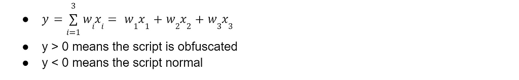
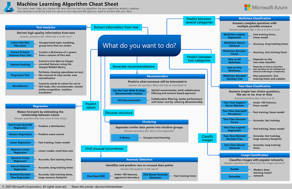
Machine learning allows us to take a bunch of samples and algorithmically find the optimal weights (or coefficients wᵢ) for this equation. “Optimal” can mean a lot of different things, but that’s the general idea. A machine learning model can be implemented in a number of ways based on the type of problem you’re tackling (e.g., Naive Bayes, Logistic Regression, Support Vector Machines, Random Forests, etc.) If the names of these algorithms sound like Greek to you and you’re interested in learning more, check out this set of posts that cover a lot of the basics. Actual models for machine learning are more complex than this toy example, but hopefully this gets the point across. There are a lot of models to choose from, which can be confusing when you’re starting machine learning. Microsoft has a great cheat sheet that highlights common approaches:​​

This toy example is an example of supervised learning, which we detail more in the following section. Supervised learning can be used for regression (i.e., predicting a numerical value, like housing prices) or classification (i.e., predicting a label like normal/obfuscated).

Types of Machine Learning Approaches

There are several ways to group machine learning algorithms, but here we’re going to use the supervised, unsupervised, and reinforcement learning buckets.

Supervised Learning

With supervised learning your data is labeled (e.g., script₁ is obfuscated, script₂ is normal, and so forth). We then extract a known set of features (such as size, average string entropy, and number of strings present in the script) from each sample, which in almost all cases need to result in some set of numbers. The data is then split into two or more sets, a training set and a test set. An approach (Random Forest, Logistic Regression, Neural Network, etc.) is then applied to the training data set to generate a model which is then compared to the test set. A number of different metrics are used to determine a “good” model based on the type of problem the model is attempting to solve.

The reason we use training and test sets is to prevent a model from overfitting the data. Overfitting occurs when a powerful enough machine learning model effectively “memorizes” the data they’re trained on but fails to generalize well on new unseen data. A model’s “power” is its capacity to represent the data it’s modeling, such as the number of trees in a Random Forest or the number of layers and neurons in a Neural Network. Finding the balance between overfitting and underfitting (i.e., when the model isn’t powerful enough to represent the data well) is one of the main challenges in building predictive machine learning models. Related to training and test sets is the concept of “K-fold cross-validation”. As a brief summary, this involves using iterated slices of a dataset to evaluate model performance metrics which are then averaged together. We see how K-fold cross-validation is used later in this post when optimizing models.

Sidenote: Getting large amounts of good and accurately labeled data is also one of the biggest challenges in machine learning! You’ll see some of the challenges of this in the Dataset Improvements section.

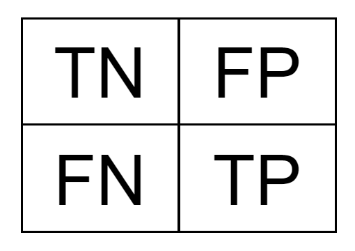
One last conceptual thing to cover: classification metrics. We need a way to compare how well each model performs on the test set they were measured against. Before we get to the metrics though we need to know about the “confusion matrix,” which is a way to summarize prediction results:

The above confusion matrix is the original Revoke-Obfuscation model’s performance on an augmented dataset (which we’ll cover in a few sections). There are different ways to visualize this matrix, but it neatly displays the correct and incorrect predictions for a particular dataset from a given model. The top left and bottom right are the number of true negatives (TN) and true positives (TP) respectively, while the top right and bottom left are the number of false positives (FP) and false negatives (FN), respectively:

There are a number of single-number metrics used for comparison classification algorithms that are derived from this table, and which one you care most about depends on the exact type of problem you’re trying to solve, how balanced the label classes are, and other factors. The metrics we’re going to focus on are:

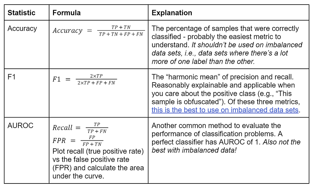
This post has a great comparison of Accuracy vs F1 vs AUROC.

Here our dataset is balanced, so which metric should we use? The answer appears to again be “it depends” ¯\_(ツ)_/¯ I ended up tracking all three of these metrics for the models I evaluated, since my knowledge of the math isn’t quite sufficient to definitively know which should be solely used in this situation. Throughout this post I use accuracy for comparison of algorithms in this post because:

a) It’s very easy to understand and

b) our dataset is balanced.

I also break out the raw number of false positives and false negatives for each winning algorithm. Security practitioners, particularly defensive analysts, are painfully aware of the “false positive problem” that plagues detection work. Too many false positive alerts can result in wasted work and alert fatigue for analysts, harming the effectiveness of a detection. On the flip side, over-reducing the number of false positives could introduce an intolerable number of false negatives. In a perfect world the model makes no mistakes, but in reality there’s an inherent tradeoff between false positives and false negatives. Which one you prefer to minimize is going to be situation dependent, which can affect the specific model you choose and/or how you tune it.

Unsupervised Learning

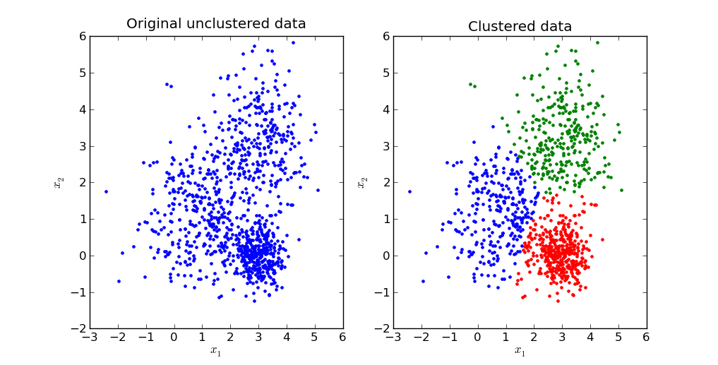
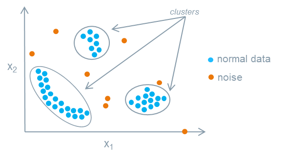
Unsupervised learning uses unlabeled data. You might ask “what can we learn from a model trained on data that’s not labeled?” which is a reasonable question. The main applications are clustering (i.e., group all of these scripts into 5 main sets), and anomaly detection (i.e., finding outliers/anomalies in network traffic). This is often harder than supervised learning because there’s often no “right” answer, but it can provide a lot of use in specific applications.

I won’t be covering unsupervised learning in these posts, but will likely cover some unsupervised learning applications in the future.

Reinforcement Learning

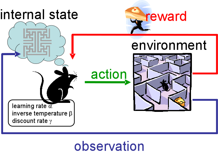
Reinforcement learning is a bit different, in that it doesn’t really use data at all! Reinforcement learning uses an “agent” that “lives” in an environment. The agent performs actions in the environment and receives feedback/rewards. Think of teaching an algorithm to learn to play Super Mario Bros., where dying provides negative feedback and passing a level earns a reward. Reinforcement learning is used to learn long-term, sequential problems like video games, chess, logistics/scheduling problems, etc. It can actually outperform humans in some cases (like AlphaGo)! I also won’t be covering reinforcement learning in these posts, but hope to return to it at some point in the future.

Visualizing the Decision Boundary

We’re going to revisit our toy example, as supervised classification problems are extremely common and are a bit easier to visualize.

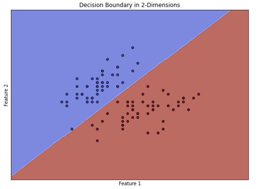
Let’s first measure two features about our labeled scripts and graph them, where red points are obfuscated and blue points are benign. We want to separate these points as best we can into two groups, so when a new unlabeled sample comes in, we classify it correctly. The line we draw to separate these two classes of points is known as the decision boundary and how this line is determined depends on the type of model we use. In the image below, we see a decision boundary drawn across the diagonal, where those points in the blue region are classified as one thing, and those in the red are classified as another:

But we’re not restricted to just two features (and therefore dimensions)! Let’s say we measure three features about each sample, which we can plot in a 3-D space. In this case our decision boundary is going to be a 2-D plane:

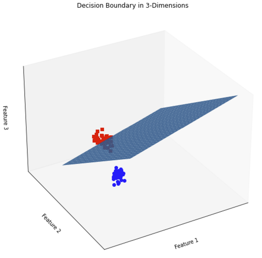
Now we can certainly measure more than three features, but unfortunately we humans can’t visualize higher dimensionality than three dimensions. Suffice to say that the math does work, and the decision boundary becomes a multi-dimensional hyperplane that divides the points in higher dimensional space.

tl;dr: ML classification algorithms turn a bunch of samples into numbers and use them to fit a giant curve/hyperplane in high-dimensional (4D+) space. This curve separates your samples into two or more classes. You use this curve to predict the labels for new samples.

A lot of what I’m going to be talking about is effectively building this highly-dimensional decision boundary on practical data sets. The following posts in this series will cover attacks that attempt to move points from one point on the decision boundary to another.

This was just a brief taste of machine learning — if you’re interested in pursuing this space beyond what I cover in this point, check out the References section at the end of the post.

Now let’s check out a practical security-related example.

Revoke-Obfuscation

Back in mid-2017, Daniel Bohannon (@danielhbohannon) and Lee Holmes (@Lee_Holmes) released an awesome body of work known as Revoke-Obfuscation. Daniel was the author of the well known Invoke-Obfuscation PowerShell obfuscation project, and the Revoke-Obfuscation work is an implementation of a machine learning algorithm trained on various PowerShell Abstract Syntax Tree (AST) features extracted from a subset of the PowerShellCorpus they collected. Their project README has some information on the background of the project in their own words, and the following resources give some more information on this awesome project: blog post, whitepaper, Black Hat USA slides, BlackHat USA presentation. They also have a great writeup on their data science approach in the repo, which is as follows:

1. Prepare a PowerShell Corpus
2. Label items in the corpus as Obfuscated / Not Obfuscated
3. Identify a feature set for the PowerShell scripts
4. Run a Logistic Regression against this corpus given the identified features
5. Export the trained feature weights to incorporate into the Revoke-Obfuscation cmdlet itself

Note: Obfuscated PowerShell is not necessarily malicious PowerShell, and not all malicious PowerShell is obfuscated! The detection of malicious scripts/binaries is a much more complex problem that often needs additional context to determine intent. Revoke-Obfuscation and this post stick purely to the obfuscation detection problem.

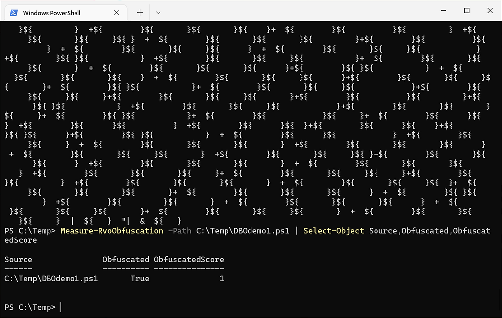
The presentation and whitepaper in particular did a great job of introducing machine learning to security professionals. It details the rationale behind the dataset construction and algorithm selection, and serves as a good documentation of the general problem of obfuscated PowerShell code. The final result is a PowerShell script that contains the trained model which can be used to examine local scripts as well as remnants in the event log:

I want to emphasize that this work was really groundbreaking for the infosec community, and many formal academic papers have since used the collected PowerShellCorpus and cited Daniel and Lee’s work. That said, after being immersed in this problem for some time I have a few criticisms that I sought out to document and improve upon for the project:

1. The PowerShellCorpus is not completely “clean”, nor is it even completely PowerShell. I only reviewed the ~10k labeled script subset used for their training and discovered a number of discrepancies that I’ll document in the Dataset Improvements section.
2. The actual labeled data set including features was not published, just the raw “Script,Label” CSV files.
3. The trained model uses a subset of data (~300 samples) from the “Underhanded PowerShell Contest” that was not published with the corpus.
4. No feature scaling (e.g., normalization or standardization) was used for applicable algorithms. This usually helps performance for most algorithms that are not tree-based (i.e. Random Forests and Gradient Boosted Trees) by compressing really large values to a smaller scale, and is usually considered a best practice.
5. The number of features (4998) was out of proportion to the number of samples (approximately 10k). There are no hard and fast rules on features versus samples, only rules of thumb. One of which is for ~10 samples per feature, so the dataset should have around ~1000 features. As evidence of this issue, approximately 30% of the feature weights for the original model published are 0, meaning those features have literally no effect on the final outcome and can be eliminated.
6. The data was a bit unbalanced, with ~6800 unobfuscated samples and ~4400 obfuscated samples (~61%/39% ratio) and steps weren’t taken to handle the imbalance dataset (e.g., additional data augmentation or over/undersampling). However this was partially due to most samples being auto-generated from a handful of tools, as there isn’t a lot of manually obfuscated PowerShell out there.

Dataset Improvements

I’ve been playing around with this project and data set for a while now and recently set out to address the concerns that I started to document.

To address the concerns with the labeled section of the corpus used for training, I manually reviewed all of the scripts (approximately 10k) the original project had labeled (remember this is a small subset of the ~300k samples in the entire corpus). This was not a fun task, but I tried to adhere to Peter Norvig’s quote of “More data beats clever algorithms, but better data beats more data.”

I found a number of interesting samples that were almost PowerShell but not technically valid (i.e., PowerShell transcription logs), some files that weren’t text at all, and some scripts in other languages (Python, VBScript, ASP, etc.), and some just raw textual data. There were also a number of duplicates which I excluded as well, along with the UnderhandedPowerShell results as we don’t have that data set. During my review, I tried to stick to “does this really look obfuscated” instead of “does this look malicious” or “should this be surfaced to IR” in order to be as “pure” as possible for the stated goal of obfuscated script detection.

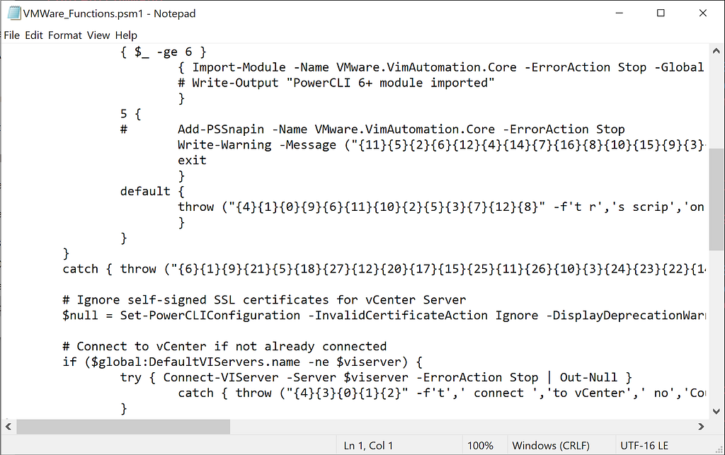
Probably Obfuscated PowerShell:

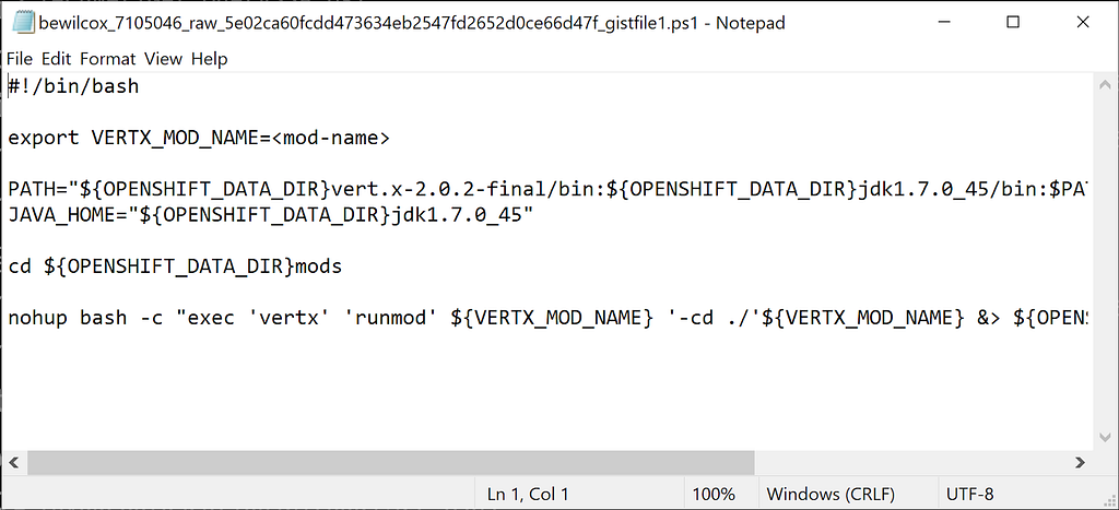
Probably not obfuscated PowerShell:

To help with the data imbalance, I took four projects/scripts that I’ve commonly used from a security standpoint (PowerView, other PowerSploit functions, PowerUpSQL, and PSReflect-Functions), extracted a number of functions from each project to standalone files (~100 total), and performed randomized runs of Invoke-Obfuscation on each. This resulted in over 1000 new samples, most obfuscated, which helped out the class imbalance.

For the lack of a fully-labeled CSV, I reimplemented the feature extraction snippets provided by Revoke-Obfuscation and regenerated the data extraction on the cleaned dataset. I am publishing the extraction code and fully labeled AST-based dataset along with all the models discussed in this post in the Invoke-Evasion repository.

The data inconsistencies I encountered were almost certainly a result of trying to gather such a large dataset and doing the labeling manually. I want to be clear that my criticisms of the dataset are not criticism of the authors- if I had created the original labeled data set I know I would have had more mistakes. In fact, I’m sure that my labeling isn’t perfect either (though hopefully it is a bit of an improvement), and some might not agree with my modifications. As always, I’m open to any feedback via new issues on the GitHub repo.

Feature Improvements

Previously I mentioned that the rule of thumb is 10 samples per feature; however, with almost 5000 features and (now) around 12k samples in the dataset, our model is in danger of overfitting itself to the data. Even if overfitting is not a demonstrably huge issue with the resulting model, not all of these features are going to be relevant in deciding if something is obfuscated. A simpler model with fewer features is preferred over a more complex one if performance is comparable, which results in faster future training and feature extraction in production. As I mentioned previously, the published Revoke-Obfuscation model had nearly 30% of the feature weights set to zero!

Given all this, I wanted to find the minimum number of features needed for the model to perform well and tried a number of approaches to do so. One motivation was for model performance, but another was a bit more nefarious: I want to know which features influence the decision boundary of the model the most, in other words which features weights are most influential for the classification decision. Or to put it in mathematical terms:

I’ll be touching on this more in the other posts in this series on attacking machine learning models, using these models as a case study.

A Baseline — Variance Threshold Feature Selection

The simplest thing we could do is see which features in the training set have zero-variance, i.e., features that have the same value across all samples (commonly 0 in this dataset). scikit-learn’s VarianceThreshold does just this:

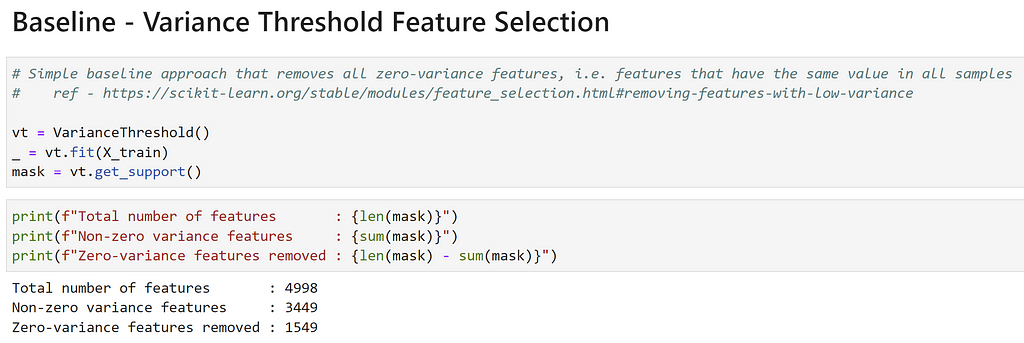
This means that 31% (1549/4998) of the features will not meaningfully contribute to any model, since they have the same values for all samples! This mirrors the results seen from the original Revoke-Obfuscation model weights. However, my gut feeling was that even among the ~3400 remaining features, many were likely very correlated or not important for the final classification decision. Let’s explore some other approaches to see how we could select the “most important” features.

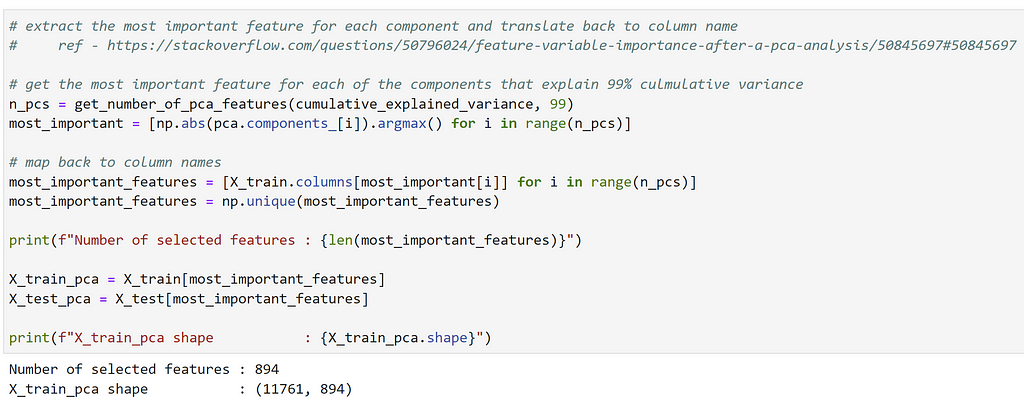
Principal Component Analysis

Principal component analysis (PCA) is commonly used for dimensionality reduction, which involves projecting a data set to a lower-dimensional space while attempting to explain most of the variance of the original data. TL;DR it’s a linear algebraic approach that extracts features from a data set that explain most of the variance in the data.

Here, I performed PCA on the training data set, and determined that ~1700 components explained 99% of the variance in the data. Taking the most important feature per component and uniquifying the list, we ended up with 894 features:

While this was interesting, it’s not what PCA is usually used for, so let’s continue our search.

Lasso Feature Selection

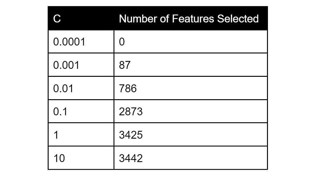
Logistic Regression models have two main types of regularization used to help reduce overfitting and improve performance on unknown data (i.e., generalization): L1 regularization (known as Lasso) and L2 regularization (known as Ridge). Without getting into the specifics of each, Lasso regularization shrinks less important model coefficients to zero, providing a type of feature selection. The hyperparameter C controls regularization strength and the following table shows the tradeoff of C versus the number of features selected:

For more details on hyperparameters see the Model Improvements section.

Retraining a fresh Lasso Logistic Regression with C of 0.01 resulted in 790 features selected (this number is slightly different from the value for C=0.01 in the table above due to the randomness inherent in the optimization process).

SelectFromModel and RandomForests

Random Forests, a type of “tree ensemble” model, have a great property that they inherently contain a measure of how “important” a feature is. This post has a good summary as to why:

…when training a tree, it is possible to compute how much each feature decreases the impurity. The more a feature decreases the impurity, the more important the feature is. In random forests, the impurity decrease from each feature can be averaged across trees to determine the final importance of the variable.

It also has a simplified explanation as well:

…features that are selected at the top of the trees are in general more important than features that are selected at the end nodes of the trees, as generally the top splits lead to bigger information gains.

If you want some more information on Random Forests or boosted tree ensembles, check out these two posts.

The scikit-learn SelectFromModel function works easily with Fandom Forests. Training a stock Random Forest on the training data, the resulting threshold/feature tradeoff is below:

With a threshold of 1e-4 we end up with 1147 features, in the same ballpark as the PCA approach and around the size we want for an approximate 10 features per sample ratio. Let’s check out a couple of more advanced methods.

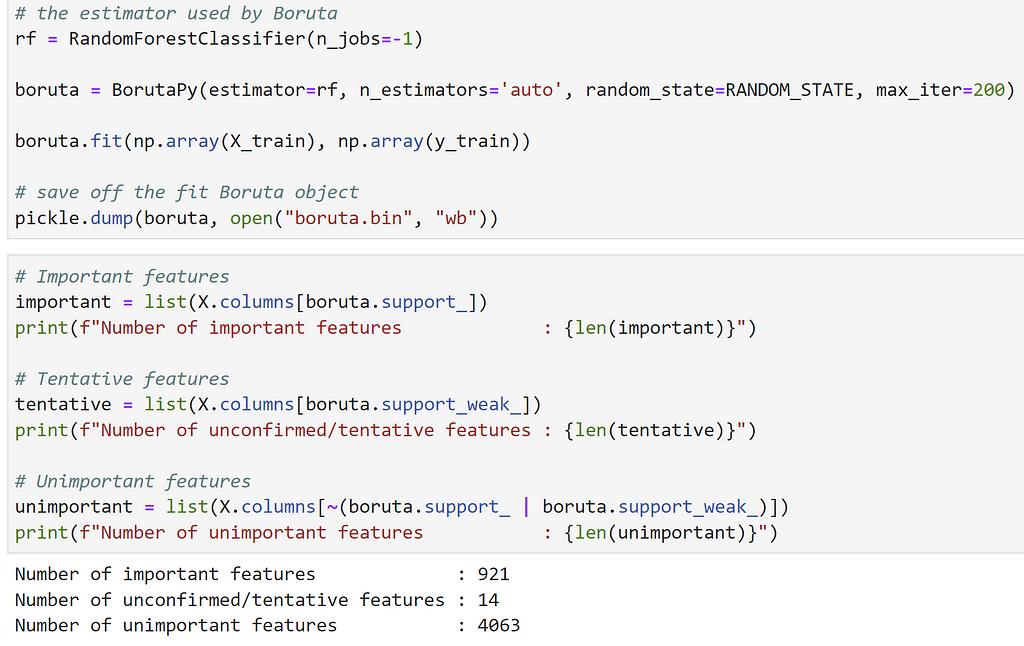
Boruta

Boruta is an “all relevant feature selection method based on Random Forest estimators” which was originally implemented in R but was ported to Python in 2015. The author of the Python port, Daniel Homola, states:

This makes it [Boruta] really well suited for biomedical data analysis, where we regularly collect measurements of thousands of features (genes, proteins, metabolites, microbiomes in your gut, etc), but we have absolutely no clue about which one is important in relation to our outcome variable, or where should we cut off the decreasing “importance function” of these.

This sounds like it might be a great fit for our high-dimensional data set! Running Boruta on the training data, we get 921 “important” features, 14 unconfirmed features, and 4063 unimportant features:

Sidenote: Boruta is a favorite of Kaggle competitions (online machine learning competitions) and is fairly “battle tested”. We’ve obviously glossed over how it works but there’s a good explanation here. Let’s check one final approach, an extension to Boruta released about two years ago.

Boruta-SHAP

Boruta-Shap is a “Tree based feature selection tool which combines both the Boruta feature selection algorithm with shapley values”. According to this post:

Boruta is a robust method for feature selection, but it strongly relies on the calculation of the feature importances, which might be biased or not good enough for the data.

This is where SHAP joins the team. By using SHAP Values as the feature selection method in Boruta, we get the Boruta SHAP Feature Selection Algorithm. With this approach we can get the strong addictive feature explanations existent in SHAP method while having the robustness of Boruta algorithm to ensure only significant variables remain on the set.

SHAP (SHapley Additive exPlanations) is a game theory approach that helps explain the output of pretty much any machine learning model. This is something that we’ll revisit in later posts when we start attacking machine learning models.

Running Boruta-Shap, we get 446 important features, 312 uncertain, and 4240 unimportant features:

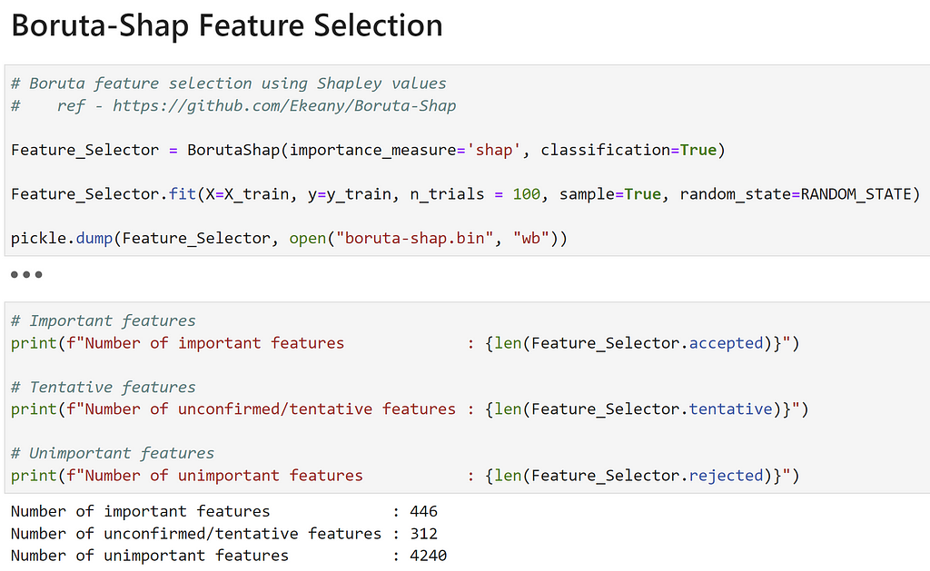
This resulted in less than half of the confirmed features as Boruta, but actually improved performance (see the next section).

Observations

I went over a lot of methods here, which might lead you to wonder, “Which selection method is the best?” I’ve learned on this journey that the answer is often ¯\_(ツ)_/¯ While machine learning is heavily built on math, from my personal (i.e., non-expert) perspective it seems like a lot of modern machine learning centers around intuition and experimentation. While there are definite guidelines as far as which architectures apply to which problems, most things I’ve seen are just that, guidelines. Datasets are all different, and experimentation is important to figure out what works best for each situation.

I felt pretty confident that some type of feature selection was necessary, based on that variance threshold baseline, the high ratio of feature dimensions to number of samples, and my general intuition about the data. I experimented with several selected feature sets, but I wasn’t able to experiment with every data set for every hypertuning approach described in the Model Improvements section.

So my approach was to take the various distilled feature sets and use them for a RandomForestClassifier and base Neural Network architecture. Overall, the Lasso, Boruta, and Boruta-Shap approaches worked the best, with those approaches very very close to each other and BortaShap ultimately edging out the others. As BortaShap also produced the fewest number of features, I took Occam’s advice and used that set of 446 features when training the various model architectures described in the Model Improvements section.

While this approach to feature minimization increased the accuracy on the data set these models were trained on, one risk is that you might eliminate features that could be important for new, unseen training data. For example, if someone implemented an obfuscation framework that functions differently than Invoke-Obfuscation, features that could be relevant for those samples may have been eliminated.

The Jupyter notebook for all this is the FeatureSelection.ipynb notebook in the Invoke-Evasion repository.

Model Improvements

Logistic Regression makes perfect sense to start with for classification. In the Revoke-Obfuscation presentation and whitepaper, Lee and Daniel mention:

For both the “In the Wild” and “Deep” data sets, this implementation gets nearly identical results to the Azure Machine Learning implementation of Logistic Regression. Boosted Decision Trees produce similar results, while the Perceptron and Support Vector Machine approaches performed much more poorly on this data set.

However, as Daniel and Lee did not publish these models nor any associated metrics, my goal was to redo an assessment of various model types. In my experiments, I wanted to try other classification model types for a performance comparison. For future posts on attacking machine learning models I wanted to have fully-explainable, somewhat explainable, and not-so-explainable architectures. I experimented with various regularizations for a LogisiticRegression model, three of the most popular tree-based models (RandomForest, XGBoost, LightGBM), and various fully-connected Neural Network architectures. For frameworks, I used what I am familiar with: scikit-learn for shallow algorithms and Keras for any deep learning architectures. For a brief tour of some common machine learning algorithms check out this post.

For each non-deep learning model, various hyperparameters were tested using 5-fold cross validation for random hyperparameter searching via RandomizedSearchCV. With the tree-based algorithms, further tuning on the most performant algorithm (LightGBM) was done using Optuna and grid searching for the LogisticRegression winner. For the Neural Network, KerasTuner was used for hyperparameter searching as well as some manual grid searching. The best model instance for each architecture was evaluated using a proper test set that was split off before any processing, with a train/test split of 80/20 (another rule of thumb). I also experimented with both normalization (MinMaxScaler) and standardization (StandardScaler) on the training input data where appropriate (all non-tree based algorithms).

Sidenote: WTF is a hyperparameter?

Model parameters are internal properties learned by the model during training. For example, these would be the coefficients/feature weights for a Logistic Regression, or the weights in a Neural Network that define the model. Hyperparameters are configurations for the model that aren’t learned directly from the data, so we manually supply them to the algorithm. Examples are the amount of regularization (e.g., C for a Logistic Regression the Feature Improvements section), the number of trees in a Random Forest, the number of layers in a Neural Network, or the exact “solver” used (the algorithm that guides the optimization process). Experimentation with a particular model’s hyperparameters to improve performance is known as model tuning. For more information on model parameters versus hyperparameters check out this post.

All of these models and Jupyter notebooks are now published in the Invoke-Evasion repository. Now let’s get into the results!

Original Revoke-Obfuscation Model

For comparison, I used the weights from the Revoke-Obfuscation model to instantiate a scikit-learn LogisticRegression instance:

lr = LogisticRegression()

lr.coef_ = np.array([[-4217.0000, 4076.5585…])

lr.intercept_ = -218.9926

lr.classes_ = np.array([0, 1])

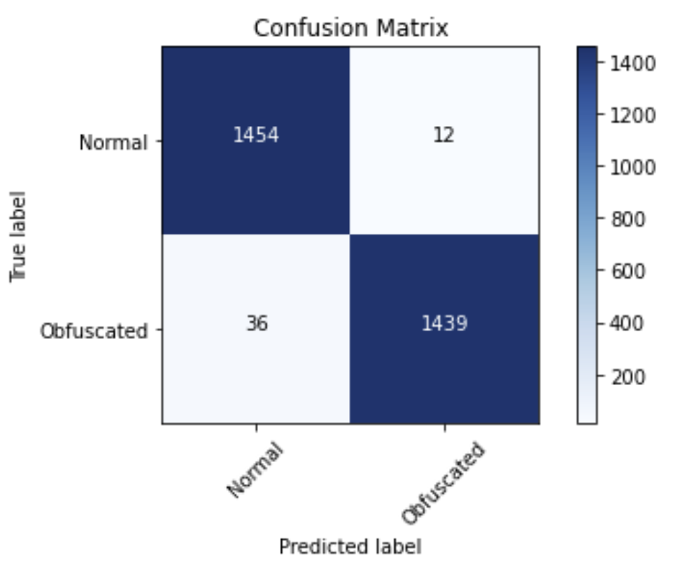
On evaluation of the newly augmented data set, this model gave the following stats and confusion matrix:

Accuracy : 0.9691

F1 : 0.9693

AUROC : 0.9690

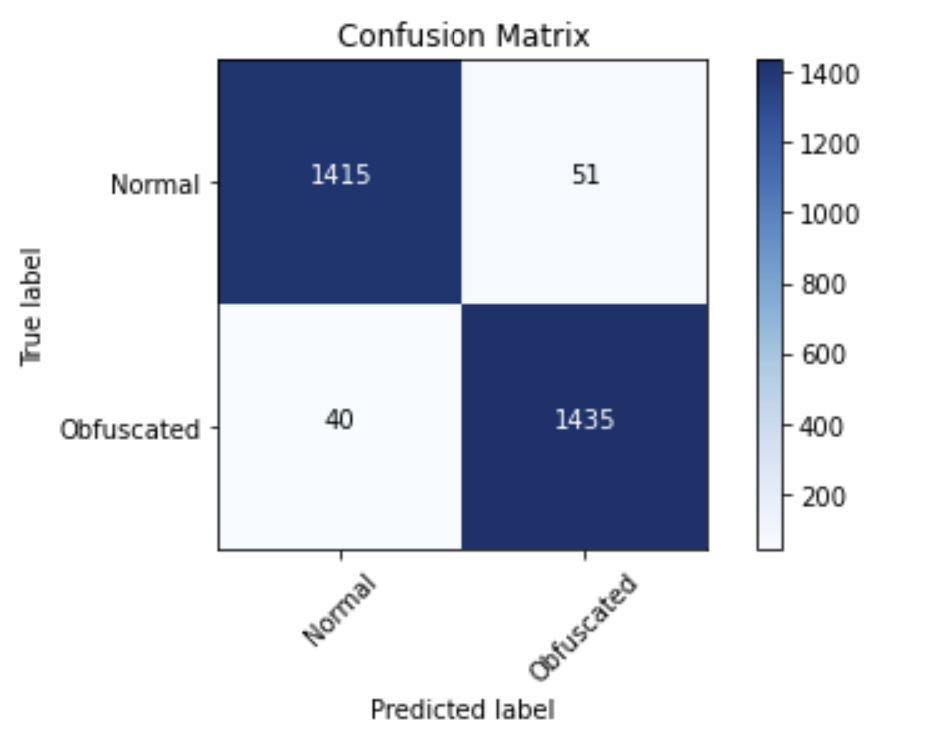
This looks like pretty good performance, and will be our baseline for further comparison. Raw accuracy is not everything, but it still does matter- see the Observations section for more discussion on this. Let’s see how additional models perform against this baseline (remember that all models from here on out will use the minimized Boruta-Shap selected feature set of 446 features).

The recreation of the Revoke-Obfuscation model is in the LogisticRegression.ipynb notebook in the Invoke-Evasion repository.

Logistic Regression

For Logistic Regression models, I used a base LogisticRegression, LogisticRegression with L1 (Lasso) regularization, LogisticRegression with L2 (Ridge) regularization, and LogisticRegression with ElasticNet regularization. For hyperparameters, I searched solvers (liblinear, lbfgs, saga, etc.) as appropriate, log10 values for C, L1 ratios for ElasticNet and StandardSaler/MinMaxScaler using a randomized cross-validated search with 5 folds via RandomizedSearchCV, and GridSearchCV to tune the winning model.

The best Logistic Regression model was a Ridge/L2 LogisticRegression with the Saga solver and C=5, trained on the Boruta-Shap set of features. It has evaluation, and confusion matrix:

Accuracy (test) : 0.9786

F1 (test) : 0.9784

AUROC (test) : 0.9939

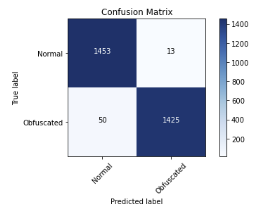
This tuned Logistic Regression in particular, greatly reduced the number of raw false positives versus the original baseline model (13 vs 51, respectively), but it did increase the number of false negatives versus the baseline (50 vs 40, respectively). This is something to consider when choosing which model is the most appropriate for production.

The experimentation with additional LogisticRegression models is in the LogisticRegression.ipynb notebook in the Invoke-Evasion repository.

Tree Models

For tree-based models (Random Forests and boosted trees), I used three of the most popular model types: a RandomForestClassifier from scikit-learn, along with XGBClassifier and LGBMClassifier boosted tree models. Like with the Logistic Regression approach, I searched for common hyperparameters using RandomizedSearchCV, but then used Optuna to better search the hyperparameter space for the best tree model.

The best tree-based model was a LGBMClassifier, with the following hyperparameters, evaluation, and confusion matrix:

LGBMClassifier(bagging_fraction=0.9095072462806773,

bagging_freq=13,

feature_fraction=0.49054439641064074,

lambda_l1=7.136741225133361e-06,

lambda_l2=1.6116201177123977e-05,

learning_rate=0.08750550951125344,

min_child_samples=91,

num_leaves=146)

Accuracy (test) : 0.9867

F1 (test) : 0.9867

AUROC (test) : 0.9980

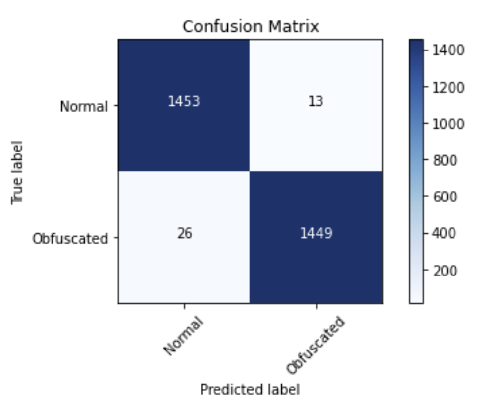
The experimentation with additional tree model architectures is in the TreeModels.ipynb notebook in the Invoke-Evasion repository.

Neural Networks

For Neural Networks, I stuck to a general fully-connected, feed-forward approach due to the tabular nature of the data. I used KerasTuner’s RandomSearch to search through a number of layers, layer sizes, dropout sizes, and learning rate combinations. I also experimented with the number of layers with a manual grid search, along with dropout and early stopping to help control overfitting. If all of these terms are Greek to you, check out the References section at the end of the post.

The best Neural Network architecture from my experiments ended up being:

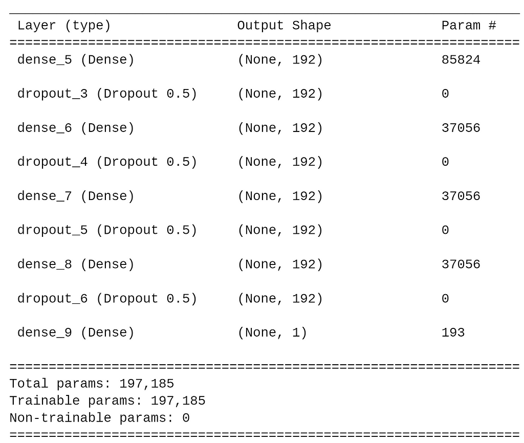
The optimizer I used was Adam with a learning rate of 0.0001, and Relu was used for the activation function. This architecture had the following following evaluation and confusion matrix:

Accuracy (test) : 0.9840

F1 (test) : 0.9840

AUROC (test) : 0.9956

The experimentation with additional tree model architectures is in the NeuralNetworks.ipynb notebook in the Invoke-Evasion repository.

Observations

This chart shows the performance for the best tuned model of each class, evaluated on the test set (2941 samples):

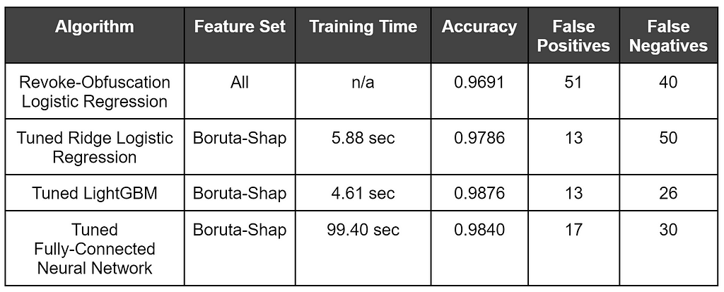
As somewhat expected, tree-based approaches generally outperformed the Logistic Regression models, with LightGBM winning out. What may seem somewhat surprising was that a Neural Network approach wasn’t really able to beat out the boosted tree model. However, despite Neural Networks being seen by many as a holy grail in machine learning, gradient boosted trees tend to outperform Neural Networks on tabular data. I also don’t have a large amount of experience tuning deep Neural Networks and I expect that others with more experience can squeeze out a bit better result.

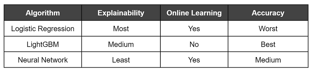
The performance for each winning model was fairly close, so why use one model over another?

Accuracy is important, but it doesn’t mean everything. In many cases a false positive might matter more than false negatives, or vice versa. If we were to use this in actual production, the false positive problem is a very real thing to consider to prevent alert fatigue/overload in analysts. If we’re using the model as a layered defense, we would likely want something that erred more on the side of reducing false positives. But if we were doing IR triage we might prefer to minimize false negatives to ensure we didn’t miss any sample.

Another issue for production is whether the model can be iteratively trained on additional data (known as online learning, versus batch/offline learning where the algorithm has to be retrained on the entire data set). Imagine this model is deployed to production in an environment, and after a period of time we get a number of false positive and false negative results, which we realize since we have a human in the review loop. Some models, like linear models (e.g., Logistic Regression) and most Neural Networks can be trained with additional batches of data to continue tuning the existing model weights. However, tree-based models in most cases need to be trained from scratch with the entire dataset each time. This can partially be addressed with some streaming approaches like the River project, but it’s still an issue to consider.

Additionally, as mentioned previously, the feature selection I performed may or may not ultimately be a net positive when using this in production. While using the Boruta-Shap feature set increased the accuracy these models were trained on, one risk is that we might have eliminated features that could be important for new, unseen training data. For example, if someone implemented an obfuscation framework that functions differently than Invoke-Obfuscation, features that could be relevant for those samples are no longer measured. There are known knowns, etc.

A final issue, that we’ll cover in more detail in the next few posts, is explainability. That is, for a decision on a given sample, how easy is it to explain why the model chose a particular label. Logistic Regression is the most explainable, with deep learning being the most opaque, and tree-based approaches landing somewhere in the middle. This is something that we’ll be exploring in depth in the next few posts.

Conclusions

I want to emphasize again how great and forward thinking Daniel and Lee’s work was. Without the details on their data science approach and the PowerShell script corpus they put together, this series of posts would not have happened.

We covered a number of potential issues with both the data set and model architecture choices of the original Revoke-Obfuscation work, and walked through data set curation, feature selection, and building more effective models for detecting obfuscated PowerShell through a series of experiments.

The winning model for each family (linear/logistic, tree-based, and neural network) along with relevant performance measurements based on the test set (2941 samples) are displayed below:

Remember that obfuscated PowerShell is not necessarily malicious PowerShell, and not all malicious PowerShell is obfuscated! The detection of malicious scripts/binaries is a much more complex problem that often needs additional context to determine intent. Revoke-Obfuscation and this post stick purely to the obfuscation detection problem.

As mentioned, the models, datasets, and Jupyter notebooks that detail the experiments in this post are all published in the Invoke-Evasion repository. In the next posts in this series, I’m going to use these three models as case studies for attacking machine learning models. Stay tuned : )

References

• The Invoke-Obfuscation project by Daniel Bohannon (@danielhbohannon)
• The Revoke-Obfuscation project by Daniel Bohannon (@danielhbohannon) and Lee Holmes (@Lee_Holmes), particularly the data science section of the README. Also their blog post, whitepaper, Black Hat USA slides, BlackHat USA presentation on the subject.
• The “Machine learning from idea to reality: a PowerShell case study” from Joost Jansen was a great inspiration for this subject area.

Online resources for general ML are a bit all over the place, with varying quality. I’ve personally liked the tutorials on Machine Learning Mastery and otherwise I usually end up Googling various concepts that end up spanning a number of other sites.

Machine Learning Books

• “The 100 Page Machine Learning Book” is a great, fairly short overview (with some math) of most ML concepts.
• “Deep Learning: A Visual Approach” is phenomenal for intuitively grasping many of these concepts (not just deep learning specific concepts).
• “Hands-On Machine Learning with Scikit-Learn, Keras, and TensorFlow” is one of the best applied books for shallow and deep learning combined.
• “Deep Learning with Python, Second Edition”, written by François Chollet (the author of Keras) is probably the best applied Keras book.
• The “Machine Learning and Security” and “Malware Data Science” books are a bit older (2018) but good examples of security-related applications of machine learning.

For something a bit more intense, the Certificate in Machine Learning from University of Washington was an awesome (and intense!) experience, and all online. I can’t recommend it enough!

---

Learning Machine Learning Part 1: Introduction and Revoke-Obfuscation was originally published in Posts By SpecterOps Team Members on Medium, where people are continuing the conversation by highlighting and responding to this story.

*** This is a Security Bloggers Network syndicated blog from Posts By SpecterOps Team Members - Medium authored by Will Schroeder. Read the original post at: https://posts.specterops.io/learning-machine-learning-part-1-introduction-and-revoke-obfuscation-c73033184f0?source=rss----f05f8696e3cc---4