Home » Security Bloggers Network » Quantifying Risk

Quantifying Risk

by Rafael Ballestas on February 18, 2019

One of the least understood parts of a vulnerability is the risk it
poses to the target. On the client side, it tends to get confused with
impact and occurrence likelihood, due to devices like the so-called
“risk matrix”, which are supposed to help us better understand
risks:

Risk matrix

Figure 1. Risk “matrices”. Via
Safestart.

Discrete scales such as this have the obvious disadvantage that they
can’t be added or mathematically operated with in a sensible way; they
can be compared, but only crudely: how do 3 lows and 4 mediums compare
to 2 highs? It is also hard to turn any of these into money terms.

While in other sectors, like insurance and banking, risk is measured
quantitatively and thus converted into dollars and cents, we are content
with leaving the treatment of security threats, basically, to chance, by
using these inaccurate scales for scoring risk.

But better methods exist in actuarial
science, statistics,
game theory, and decision
theory, and they can be
applied to measure cybersecurity risk.

Among the main reasons why these methods are not widely accepted in the
field are:

Security breaches are rare, so we can’t possibly have enough data to
analyze. It wouldn’t be “statistically significant”.
We do not see how we can measure risk, or even understand what
measuring is nor what it is that we want to measure, nor how.

Before going into ground definitions, let me show you what we can
achieve by applying quantitative methods to risk measurement:

Loss Exceedance Curve

Figure 2. Loss Exceedance Curve ^[1]

This curve tells you the probability of losing any amount of money or
more. Thus from the graph, we can read that the probability of losing
$10 millions or more is around 40%, but losing more than $100 is
unlikely at around 15%. You can enrich it with your risk tolerance
(what is the probability that you can accept to lose n millions?) and
the residual risk shows how the risk is mitigated by applying some
controls. With this kind of tools, you can make more informed decisions
regarding your security investments. If such a level of detail interests
you, please read on.

Measuring requires specification

First, we need to define what we want to measure. Is it possible to
measure the impact of a breach on my company’s reputation? Is reputation
even measurable? What makes some things measurable and others not? Well,
we need to be able to assign a number to it. But also no measurement can
represent reality or nature with 100% accuracy, so there must be some
uncertainty in measurement. Uncertainty is inherent to measurement.

In the lab, the length of an ant could be reported as 1.2 cm plus or
minus 0.1 cm, which yields an interval: the real size of the ant is
somewhere between 1.1 and 1.3 cm. There might also be some error due to
random mistakes or improper use of the measuring device, so we can
assign a confidence of, say, 90%, to this measurement. Observations
reduce the uncertainty in a quantitative way. At first, we might have
estimated the length of the ant to be between, say, 0.5 and 3
centimeters, with 60% confidence. After measurement, we have less
uncertainty.

Thus, what we think is intangible or unmeasurable could actually be
measured. Continuing with the reputation example, this might be measured
indirectly by the drop in sales, or by the costs incurred in trying to
repair the reputation damage. Another possibility for measuring could be
decomposing the problem into smaller ones. For example, instead of
trying to directly estimate the cost of a security breach, you might
break it up into affectation to confidentiality, integrity, and
availability. How many records could be stolen or wrongfully modified?
What is each of them worth? For how long could our servers be out of
service? How much money would be lost per hour?

Furthermore, events like these need to be time-framed. It doesn’t make
much sense to ask “how likely is it that our organization suffers a
major data breach?” because, given unlimited time and resources, it is
almost certain to happen. Plus, we probably don’t care if it were to
happen eons from now. We need to set a reasonable time frame, like a
year. Once we achieve a result such as

There is a 40% chance of suffering a successful denial of service
lasting more than 8 hours in the next year.
If such a denial of service happens, there is a 90% chance the loss
will be between $2 and $5 million.

We could indirectly compute what might happen in 2 or any number of
years.

Finally, there is the issue of not having enough data to perform
measurements or estimations, or rather, thinking we don’t have enough
data. That is not the case or, if it were, then the established
qualitative methods like assigning arbitrary names on a scale of 1 to 5,
are just as inappropriate or more, actually introducing noise or error.

Subjective probability

The ultimate goal will be to perform a simulation of random events, also
known as Monte Carlo simulations. This
type of simulation runs many times on single events, and their happening
or not happening is based on a probability
distribution,
and such distributions require parameters as input. These parameters
usually determine the location and shape of the curve.

Some probability distributions

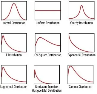
Figure 3. Some probability distributions

These parameters are to be estimated by experts, just like they estimate
risk on a scale from 1 to 5. Just as imprecise, perhaps, but the math
performed with the distributions obtained from these parameters sort of
rights the wrong in the initial guess. Actually, subjective probability
estimation can be calibrated to a point where it can be done
consistently and accurately.

Even if the estimates are completely wrong, the good thing is that they
can be further refined by a simple rule from basic probability theory:
Bayes rule. It involves the prior probabilities
(i.e., our estimates or initial beliefs) and the posterior
probabilities, the ones computed after observing a certain piece of
evidence.

Without going into details,
which we will leave for the next articles,
it can be shown that,
from five expert inputs,
including the probability of a successful penetration test,
and the probability of remotely exploitable vulnerabilities
when the pen test is positive,
that in that case,
the probability of suffering a major data breach
can go from a prior of 1.24% goes up to a resounding 24%.
If the test is negative,
it goes down to 1.01%.
This shows,
by the way,
the benefit of a proper pen test
regarding the value of information.

Later we will also discuss more advanced methods based on Bayes rule
such as iteratively adjusting distributions, which
allows making forecasts with very scarce data, and decomposing
probabilities with many conditions.

This article merely pretended to be an introduction to the whole slew of
methods that exist in other fields to estimate risk, uncertainty and the
unknown, but have not been adopted in the field of cybersecurity. In
upcoming articles, we will show in more detail how some
of these methods work.

References

R. Diesch, M. Pfaff, H. Kremar (2018). Prerequisite to measure
information security in Proc.
ICISSP 2018.
B. Fischhoff, L. D. Phillips, and S. Lichtenstein (1982).
Calibration of Probabilities: The State of the Art to 1980 in
Judgement under Uncertainty: Heuristics and
Biases.
D. Hubbard, R. Seiersen (2016). How to measure anything in
cibersecurity risk. Wiley.