Journey to the Median

One of the first problems I worked on in my recent transition from a Security Operations Analyst (SOC) to a Data Engineer at Arkose Labs, was to implement the data models and workflows for our new Customer Dashboards, which included the data for median completion times on our puzzles. This was a new metric that was being introduced — previous incarnations had displayed the arithmetic mean rather than median, but the latter was a much more useful measure and was highly requested by our customers and internal analysts alike.

I thought to myself: “Medians, how hard could that be?”

Little did I know that I was in for a most humbling and educational journey in implementing what initially seemed like such a straightforward (surely a 1-pointer) problem to solve.

First, some background

One of the statistics that we care about at Arkose Labs is the completion time on a particular Enforcement Challenge puzzle. This is usually framed in one of two ways:

• Is this challenge taking too long for our users and frustrating them?

• Is this challenge successfully wasting time and resources for fraud farms?

Our technical artists care about these questions in order to develop puzzles that have the double-edged blade of excellence: easy on human users, yet resilient against machine learning,

Our SOC team cares about these questions in order to apply the most effective puzzles for different types of attacks.

Our Product team cares about this in order to plan roadmaps for future puzzle development.

And our customers care about this to ensure they are providing a frictionless user experience for their true users.

Representations of this Measure

Arguably one of the most illustrative and informative ways to communicate information about a distribution is with a histogram:

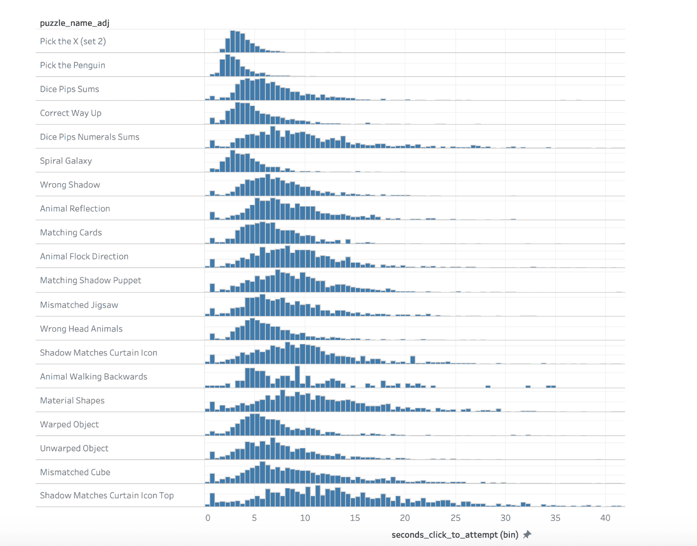
Here we show the number of sessions (y-axis) that took a certain number of seconds (x-axis) to complete a challenge, for each type of puzzle.

Something to notice in the above distributions is that there is a tendency for the distribution to be skewed. This makes sense: completion time is left-bounded (since it is not possible so solve a challenge in 0 seconds or less), and there is some variance, not only in the solving ability of different people, but also in whether someone is fully engaged with completing the challenge, or instead perhaps has gotten up to go make a coffee.

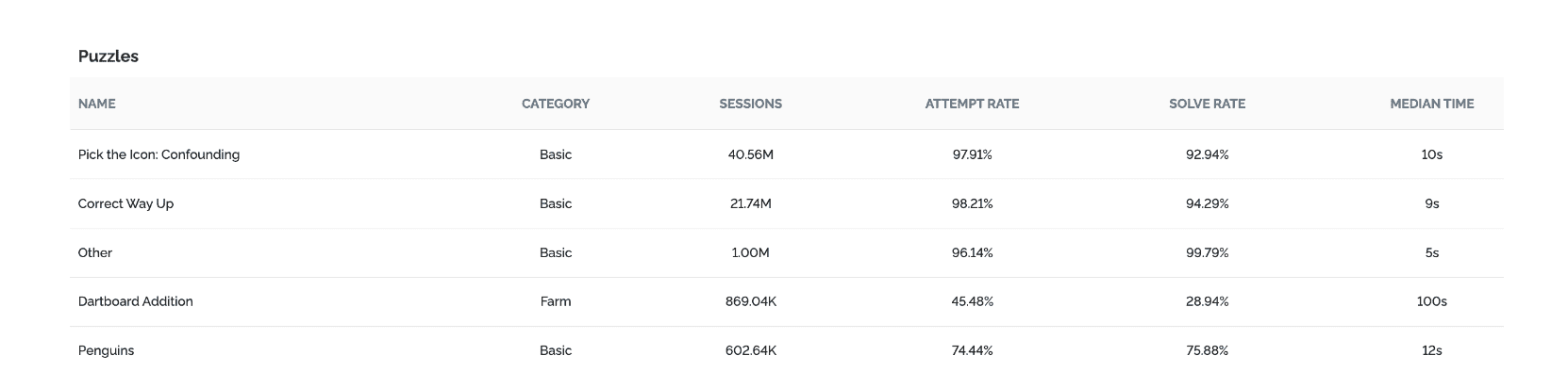
Despite the indisputable superiority of the histogram representation, it is not always ideal. In some cases, we may want a simpler, lower-resolution measure, such as a summary statistic, especially when displayed in very high-level summaries such as the Puzzle Summary Table in our Customer Portal Dashboard:

When we were designing the data for the Customer Dashboard, one initial question we asked ourselves was, what choice of measure of center do we want to display? The three obvious ones are:

• Mean

• Median

• Mode

Here are just some of the high-level considerations that came to mind with these three:

• Mean: It is O(n). Pretty trivial to implement (supported natively as a function in most if not all the major RDBMs). However, it is greatly affected by skewed distributions such as the one we’re dealing with.

• Median: It is.. probably O(n log n)? Linear solutions seem to exist for approximations, but that requires further research. Some RDBMs support a percentile or median function natively, including the one we would use (PostgreSQL).

• Mode: Looks like also O(n log n). It is the least affected by skewed distribution. Might be simple to implement, needs more thought. However, multi-modal and sparse datasets might be a challenge. Very flat distributions may also create misleading results.

The real trouble with median

At this time, I was not yet aware of the real problem with median, which I only came to understand much later. In fact, it was during the writing of this blog post that I actually sat down and thought about it for its own sake, googled some things, and was finally given a name to the idea I had in my head (thanks to my indispensably talented colleague Dimitri Klimenko for immediately grasping my poorly-articulated ramblings and finding the concept for it): Decomposable Aggregate Functions.

In this period of my youthful ignorance, I had assumed median would be somewhat similar to implement as mean. Isn’t it just another measure of centre, another summary statistic? Why should it be significantly different?

What I quickly realised was that median doesn’t aggregate very nicely. Consider a function like max(). Suppose I’ve already computed the maximum completion time for some Puzzle A and the maximum time for some other Puzzle B. Now I want to know the maximum completion time for both Puzzle A and B. Well, that’s just the maximum of the two maxima:

Similarly, consider the function sum(). I’ve got the sum of salaries in the Data Science team, and the sum of salaries in the Data Engineering team. To get the combined payroll expense for both Data Science and Engineering teams, that’s just the sum of the two sums:

The situation is similar for a few other functions like count(), min(), average() (arithmetic mean). Mean is marginally more complex because it involves keeping track of both the numerator and the denominator in order to re-calculate the aggregates, but we can still compute the aggregates for separate sets and then merge the results together to get the average for the entire set.

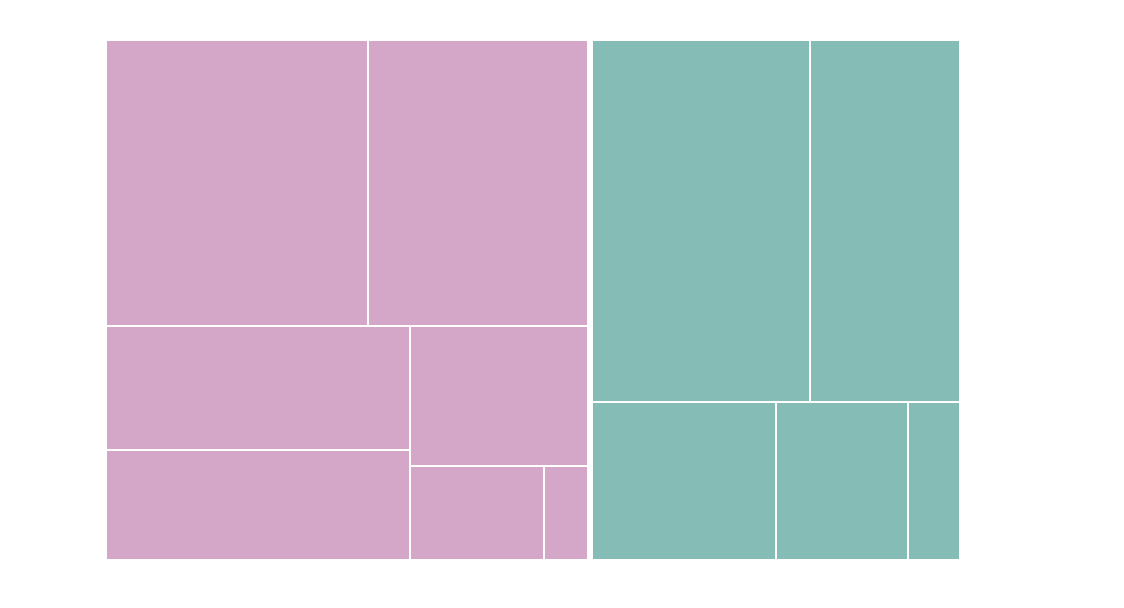
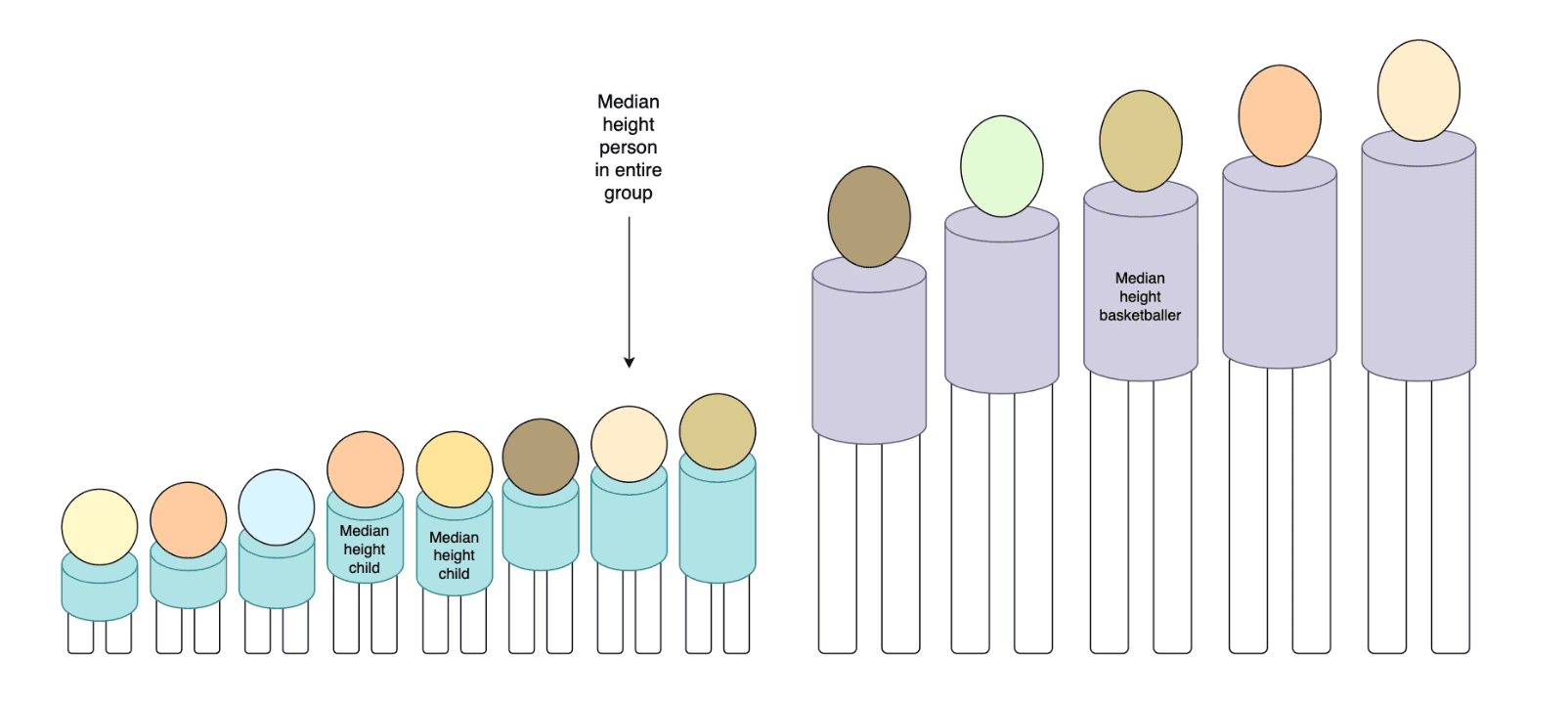
However, median does not play nicely like this. Having the median height of a kindergarten class and the median height of a basketball team tells me nothing useful about the median height of the combined group of both the kindergarten children and the basketballers:

I have to keep the more granular, underlying data points in order to compute the median, and there didn’t seem to be any really obvious way around it, short of thinking really really hard, or reading really really hard theory papers (neither of which I ended up doing).

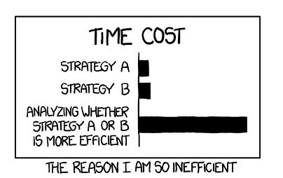
What I did end up doing is trying random stuff until it worked. Admittedly not the optimal strategy in retrospect, but one that feels sensible when you incorrectly assume the problem you are solving is very simple and that you are always just an hour away from success. Here’s a recount of the journey:

Stage 1: Store the data raw, compute it at query time

This is the obvious, naive solution. The problem is that one of the requirements for the Customer Dashboard is to be able to display data for the past 90 days.

90 days of data at Arkose Labs means around 4.5 billion sessions, and we weren’t about to go ahead and store 4.5 billion records in our Postgres table.

We must go deeper!

Stage 2: Store the data aggregated, compute it at query time

Instead of storing session-grain data, let’s try the more reasonable thing of aggregating our data by timestamp. What should our time grain be?

We had another requirement that the Customer Dashboard should be able to display data for the past 24 hours. Now “last 24 hours” does not mean “yesterday, from midnight to midnight”, rather it means from this time 24 hours ago, until now. We had already decided that our data workflow jobs would run on a schedule of once every 10 minutes. So, we need to support at least a 10-minute granularity of data in order to be able to allow accurate filtering to the last 24 hours.

What is the expected size of our table now? Here are the dimensions we are dealing with:

• 90 days * 24 hours/day * 6 intervals/hour = 12,960 time partitions

• 60 puzzles

• 300 x 3 x 2 other dimensions

This comes out to ~1.4 billion possible unique combinations, and we haven’t even added any dimension for completion_time yet.

Suppose we choose a 1-second grain for completion time (in our raw data, we store it at millisecond precision), and suppose we exclude any values greater than 10 minutes. This comes out to 600 unique values for completion time.

600 * 1.4 billion: I need not perform this simple arithmetic to know that this is already multitudes worse than just storing the raw session data for 4.5 billion records.

However, it is very unlikely that we actually have all 60 puzzles seen across all of these 300 x 3 x 2 mysterious “other dimensions” in every single 10 minute interval in a 90 day period. The real projection should be significantly smaller (for example, some puzzles are exclusively used for the purpose attack mitigation and never during peacetime).

A rough analysis on some data shows that the real projection is around 7.8 billion. However, this is still worse than just storing the raw data.

We must go deeper.

Stage 3: Store older data at lower granularity

Going back to the requirements for time filtering for the dashboard, these were the filters we needed to support:

• Last 24 hours

• Last 7 days

• Last 30 days

• Last 90 days

• Custom (day grain: midnight to midnight)

I’d argue it’s a reasonable compromise to treat the “Last X Days” with a little less precision than “Last 24 hours”, and equate them with being a custom time range from midnight to midnight.

In this case, the 10 minute granularity of the data is only needed for the “Last 24 hours” filter. For all the other filters, we only need data at a day grain. This should reduce the data size by at least 144-fold. We’re now at 50 million records, which is still not great, but worth a try.

Stage 4: Implementing a median function

Since we’re pre-aggregated our data, we’ve lost access to the underlying raw values and therefore can’t use PostgreSQL’s native percentile_disc() function to compute the median. Instead, we need to write our own SQL to compute what we might call a “weighted” median.

Here is the SQL I ended up writing for this (other dimensions were removed for clarity):

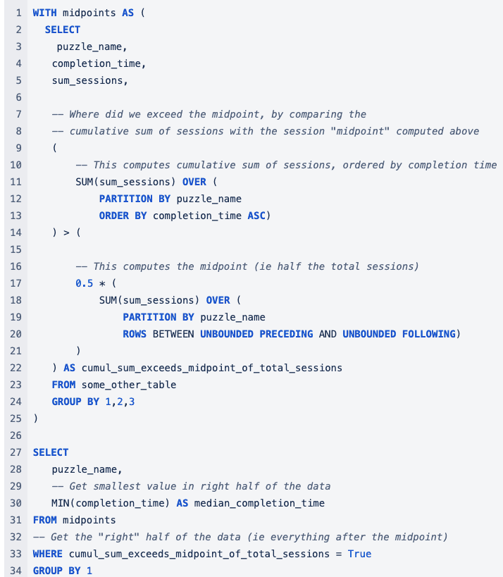
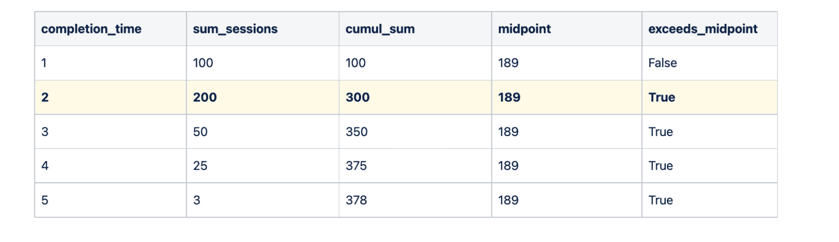
This is the intuitive solution: sort the rows by the completion time, track the cumulative sum, find the midpoint, and see where the completion time crosses the midpoint. In the below example (other dimensions excluded for clarity), our median completion time would be 2 seconds.

I prepared a sample dataset with 90 days of data at 1 day grain and ran the query. It took over 30 seconds to execute. Did I mention that one of the requirements for the Customer Dashboard was that the queries need to return in under 7 seconds?

Time to go deeper.

Stage 5: How about pre-computing the medians?

What if, instead of computing the median at the time of the query, we precomputed them in our prepared tables?

Back to my little book of rough calculations. Supporting every possible combination of the grouping dimensions means:

• 89 + 88 + … + 2 + 1 = 4005 distinct time ranges (every possible choice of a time range within the 90-day period)

• 60 puzzles

• 12 other filter combinations

We’d be storing pre-computed data for 4*4*59*4005 = 2.8 million unique groupings of the dimensions. An unpromising path.

Stage 5.5: A drought of ideas

At this point I was feeling a bit discouraged. Here were some of the fruitless ideas I thought of during that time:

We could consider a different measure of center. (Implication: admit defeat)

We could greatly increase the bin size on completion time to reduce the size of this dimension. (Implication: provide unacceptably imprecise data for customers)

We could Implement an approximate median function. (Implication: spend an unknown amount of time reading very hard papers and thinking very hard)

Stage 6: Hearing the Hansbach

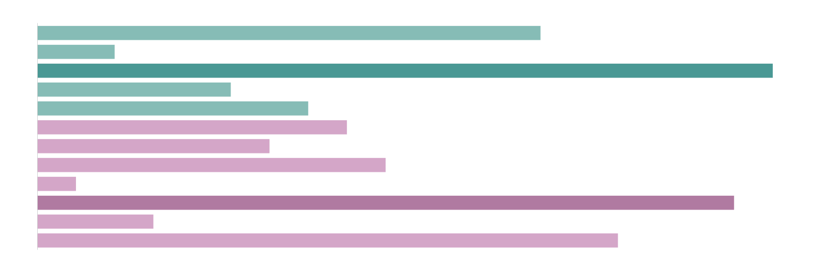
I must have scrolled idly up and down the wikipedia page for “Histogram” more than a few times during this whole endeavour. I had been staring at this image when the answer became evident.

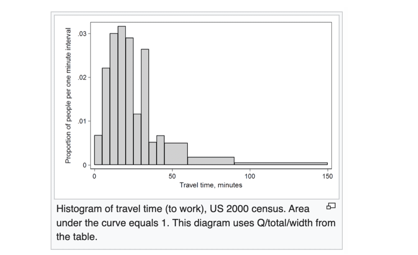
The problem is that even with 1-second bins (which is already fairly imprecise at the low end), we still had a considerable longtail of higher completion times that were contributing hundreds of unique completion_time values.

But does anyone really care about the difference between, say, 126 seconds and 129 seconds? Could we not just drop both into the “it’s around 2 minutes” bucket, since, this is probably how I’d convey this information in an informal conversation about puzzle performance anyway if I was looking at a histogram and summarising what I see (“Well, it appears most users complete it in around 3 seconds, and maybe 99% within 2 minutes.”)

Stage 7: Variable bin sizes

Next, I drafted up some very rough bin sizes that would increase with the completion time, just to see if this would improve things. I didn’t employ any kind of fancy math or try to optimise for the best choices of bin size. Mostly I was choosing numbers that would make sense when displayed and not mislead users into thinking the numbers they were looking at were more precise than they in fact were.

Here were the bin sizes I chose:

• 1-9 seconds: bin size 1 second

• 10-29 seconds: bin size 2 seconds

• 30-59 seconds: bin size 5 seconds

• 60-119 seconds: bin size 10 seconds

• 120-299 seconds: bin size 30 seconds

• >300 seconds: bin size 60 seconds

This come out to around 40 bins instead of the original 600, a further 15x reduction.

After re-running all my aggregation jobs, I re-ran the median query for all puzzles in the full 90-days time range and it ran consistently in under 1 second! Success! Finally I can give my team a different status update at tomorrow’s standup!

Back to the surface

What have I learned?

• A lot more about databases, data modelling, and SQL than I did before.

• And that I really love databases, data modelling, and SQL even more than before!

• That writing a blog post is an excellent opportunity to revisit a problem in more detail, do some research, and learn more about it.

Thank you for reading, and have a great day.

*** This is a Security Bloggers Network syndicated blog from Arkose Labs authored by Delia Wang. Read the original post at: https://www.arkoselabs.com/blog/journey-to-the-median/