From the Data Scientist’s Desk: How to Tune a Model Using Simple Analytics on the Feature Contribution Data

My story: My model looked good. It was as accurate as I wanted it to be and I was happy with it from one experiment to another. When I decided to change the test data set a bit, everything fell apart. Accuracy dropped and I had no clue why. I had to run the test again. And again. Ten tests later, I finally understood that simply restarting the test doesn’t fix data science issues, and got to work on a solution.

First, I tried to look at the misclassifications but nothing popped up. They looked different from each other. Then I decided to check the feature contribution for the different groups. This helped me find the trouble-making features and tune my model. In this post, I’ll describe in detail my experience of tuning a model using simple analytics on the feature contribution data.

Prediction and Feature Contribution

I used the sklearn predict_proba method which returns an array of predictions. I assume a trained model, and x as an input:

y = model.predict_proba(X=x)

Each prediction has a probability between 0 and 1. There are several ways to get a prediction’s features contribution. A very popular way is SHAP, which is model agnostic. Since the model I use is Random Forest, I chose to use the treeinterpreter library, for better performance. Here is a code example:

from treeinterpreter import treeinterpreter as ti
y, bias, contributions = ti.predict(model, x)

The bias is the base result for each prediction, and the contribution is a number between -1 and 1 per feature.

y = bias + SUM(contributions)

Model Debugging with Feature Contribution

All went well and the model looked good. Then when I made a small change to the data, the result was a giant leap in the number of misclassifications.

To investigate, I calculated the feature contribution on the misclassified results only. This is an important optimization since calculating the feature contribution on a large data set may take a long time. y_true hold the actual classification values:

y = model.predict(X=x)
x = x.take([i for i, val in enumerate(y_true) if val != y[i]])
y, bias, contributions = ti.predict(model, x)

Now that I have the contribution data, it is time to use it to fine tune the model.

Fine tuning a model

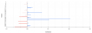
False Negatives

For false negatives I want the probability to get higher, so I will focus on features with high negative contribution. I aggregated all the data using the average function and got the following results. The red bars represent features that made the score lower (i.e., negative) instead of high. These are the features that I want to check.

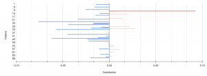
False Positives

In false positive classifications, I expect the model to give a low score, so I will focus on features with high positive contribution:

Full Features Map

As I saw, a change in the feature that caused a high rate of false positives (FPs), can influence the rates of the other three types of classification. An interesting perspective is to look at the influence of each feature on all classification types (TP, TN, FP, FN) at once.

I created a heat map using the following steps:

1. Group the data by a classification and a feature.
2. Calculate the average contribution.
3. Invert the contribution of the TN and FP groups in which I am looking for low contribution. You can find an example SQL code below.

Here are the results:

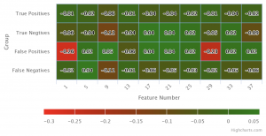
You can observe in the heat map the features performance in each of the groups. Good contributions are green and I will update / remove features with bad contributions.

Analytics Technical Details

I wanted to share an example of how I calculated the contribution analytics. Because I used a lot of data, and wanted to do multiple analytics – I chose to load the data into our data lake and use SQL on the contribution data.

Here is an example for the query I used to create the heatmap above :

WITH data AS (
 SELECT feature, classification,
        CASE
          WHEN classification IN ('FP', 'TN') 
            THEN -AVG(contribution)
          ELSE AVG(contribution)
        END AS contribution
 FROM contibutions_table
 GROUP BY feature, classification)
-- Order the data to find the top feature contributions
SELECT *
FROM data
ORDER BY SUM(ABS(contribution)) OVER (PARTITION BY feature) DESC
LIMIT 100

You can use similar queries to find information about your model’s features contribution.

The takeway lesson from this experience

Tuning of a model is a data scientist’s most difficult, or at least the most time-consuming work. Here I have demonstrated how simple analytics on the contribution data can help understanding the features performance which makes this process simpler.

My suggestion is to validate the model on various test sets and use the contribution data to learn more about the features and fix problems – it should save you time.

I believe that knowing more about the contributions will help learning both about your model and your data which will lead you to better results.

The post From the Data Scientist’s Desk: How to Tune a Model Using Simple Analytics on the Feature Contribution Data appeared first on Blog.

*** This is a Security Bloggers Network syndicated blog from Blog authored by Ori Nakar. Read the original post at: https://www.imperva.com/blog/how-to-tune-a-model-using-simple-analytics-on-the-feature-contribution-data/