

Adding Some Salt to Our Network – Part 2
How our configuration management actually works
Following a previous post which explained why we needed a configuration management system, this post explores how we built and implemented our configuration management using SaltStack. It describes the structure of our configuration and the toolset we used for modeling, automating, reviewing, deploying and validating the network configuration in our devices.
So, let’s dig into some technical details.
The pillars – and our configuration structure
As previously mentioned, it was very important for us that any configuration common across multiple devices should be written only once. Once we’d modeled out the configuration, we built it in hierarchies. At the top levels you could find the parts of the configuration that were shared among all our devices. A level below, you could locate all the configurations belonging to a specific device type, such as configurations shared between all switches, and in the level below that would be all the configurations shared by all devices from type X with role Y and so on… I’ll try to demonstrate it in a diagram, although, of course, in reality it’s much more complicated.
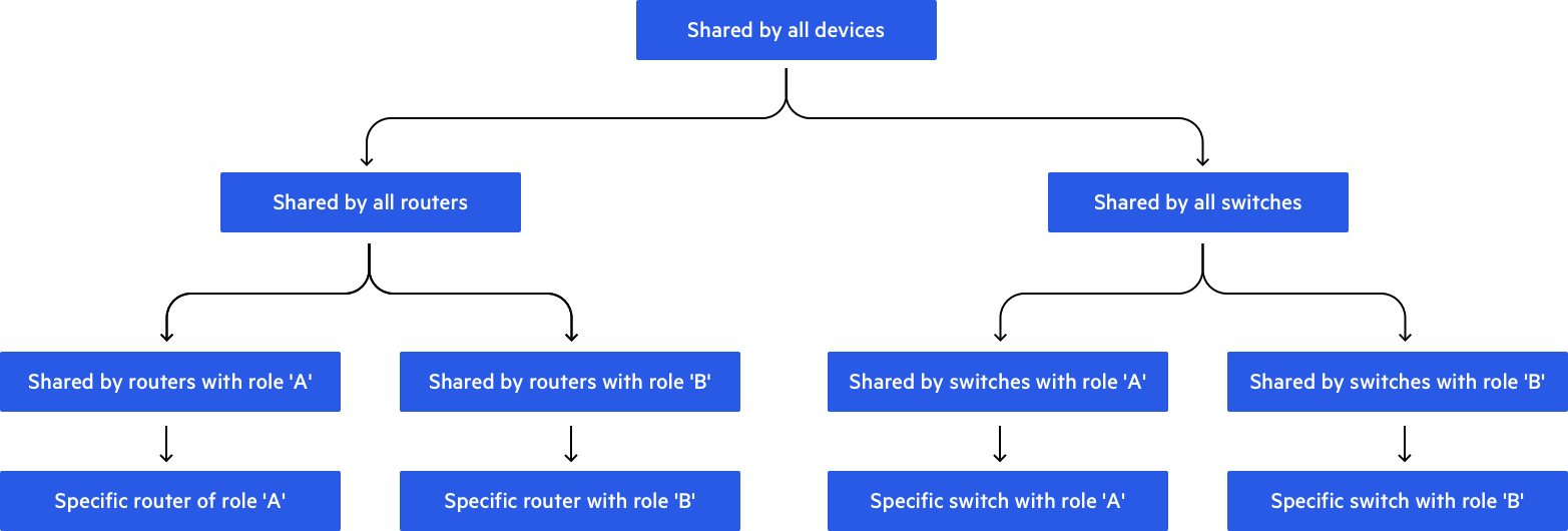
After we’d modeled the configuration in that way, we could use the pillar systems to build it out. In order to apply those hierarchies we used include statements – in the top.sls file, for example, we included the configuration pillar of the specific device; inside the device pillar we included the pillar of its father in the hierarchy tree, and so on.
Let’s see a little bit of code for a better understanding.
Our top.sls file is very simple and look like this :
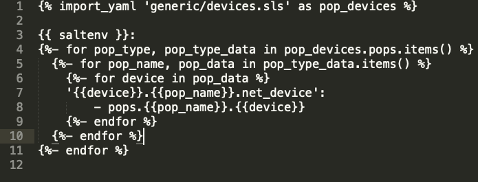
The pop_devices contains a list of devices all around the world. For each device we used only a single pillar file, in which we’d define the type of device according to the include statements inside that particular pillar. For example, the pillar file of specific router with role b includes the file of share router with role b. By doing this, it will classify itself as a router with role b.
Let’s take a closer look at our pillar directory structure:
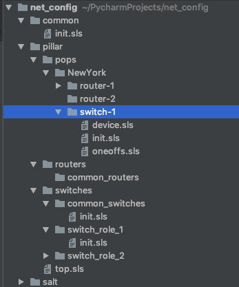
This structure represents the hierarchy shown in the diagram above . If we look again in the top.sls file we can see that the directory pops/newYork/switch-1 belongs to our device. The file pops/newYork/switch-1/init.sls will look something like:
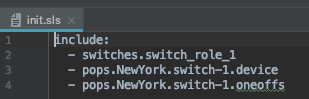
Three files are included:
- switches.switch_role_1 – including this file will import all the definitions shared by all switches which play a specific role ( role_1). By including this file we’re defining for Salt that this device is a switch from role 1.
- pops.NewYork.switch-1.device – this file contains a configuration unique to this device.
- pops.NewYork.oneoffs – in some cases we’ll need exceptions to common roles (switches/switch_role_1). Let’s assume, for example, that in all switches taking the role of switch_role_1, we have an interface towards a specific service. That kind of configuration will be described as the common configuration of switch_role_1, but if for any reason that service is not present in one of the PoPs, we’ll need to override the configuration of that service. The oneoff.sls file is used to add/remove/override parts of the common configuration.
I hope that in the point above, our configuration structure is clear. Inside the init.sls for the switch_role_1 we include the switch_common, and in the switch_common we include the configuration shared by all devices.
Applying the configuration
After building the configuration, the next step is to render the configuration to the device-specific language (e.g. vendor Config Structure) and create the procedure for applying it. For the rendering, we used Jinja2 , a common templating tool. We created Jinja templates for each part of our configuration and, on top of these, built Salt states for loading them into the device using the Salt-NAPALM module.
Jinja is a very convenient language for writing templates, although it’s not necessarily pleasing on the eye. If the template files becomes very long or too complicated you can get dizzy just from viewing them. So, in order to keep our templates maintainable we broke the configuration into many small templates – which are easier to understand and maintain.
Another thing that was important to us was to manage all device updates in a declarative way. This means that we don’t need to know what’s already configured on the device – instead we only want to declare what the desirable configuration should be. No matter what’s currently configured on the device, it should be replaced with the newly generated configuration.
Here’s an example of a template for configuration vlans. Vlans.j2 (by extending the group_base we using the template namespace):
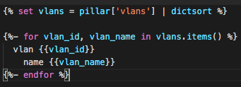
The template is actually a configuration of vlans on the device. The length of this template is 5 lines, which we believe is optimal for templates (Try to imagine how hard is to read such a template with more than 100 lines of code).
The deployment and monitoring system
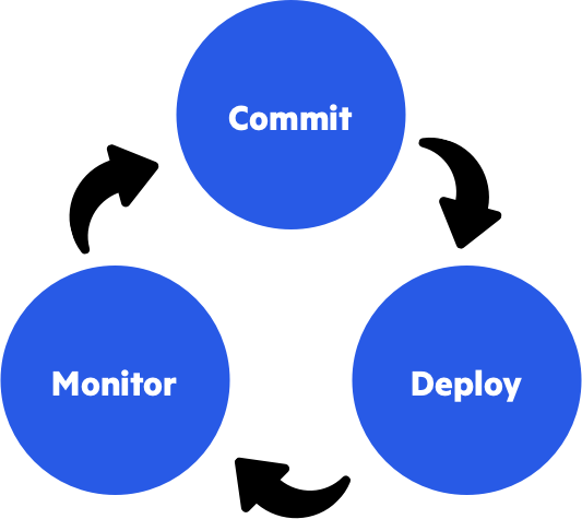
After creating the infrastructure for rendering and deploying the configuration, we must define and build a process of using it in order to commit changes, deploy to our devices, and monitor that deployment. We separate this process into three parts:
- Commit a new configuration into our codebase – a process that includes CI which validates that the new commit didn’t break anything in, as well as a manual review by other team members.
- Deploy new configuration – a process that includes a controlled deployment on our devices.
- Monitoring – check that the actual device configuration is aligned with the single source of truth in our code repo.
I’ll try to elaborate a little bit on each of the processes.
Commit of new configuration
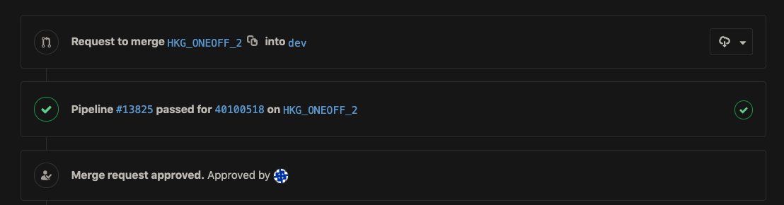
For managing our source-of-truth we’re using Git with GitLab Flow methodology. When engineers want to insert a change into production, they’ll open a feature-branch, and every time the feature is pushed into the GitLab repository a CI process will run. If the change affects only a single device we run the CI on the configuration for that device. If the change affects many devices, we choose a random configuration of one of the devices that will be affected. The CI loads the rendered configuration into the device in the lab. Then, once the configuration has been loaded, and the syntax is valid, the job will run some functionality testing.
After this we enforce another process of manual code review, and we merge it to the dev branch corresponding to the master branch in GitLab Flow. At this point the change is now ready for deployment.
The deployment process
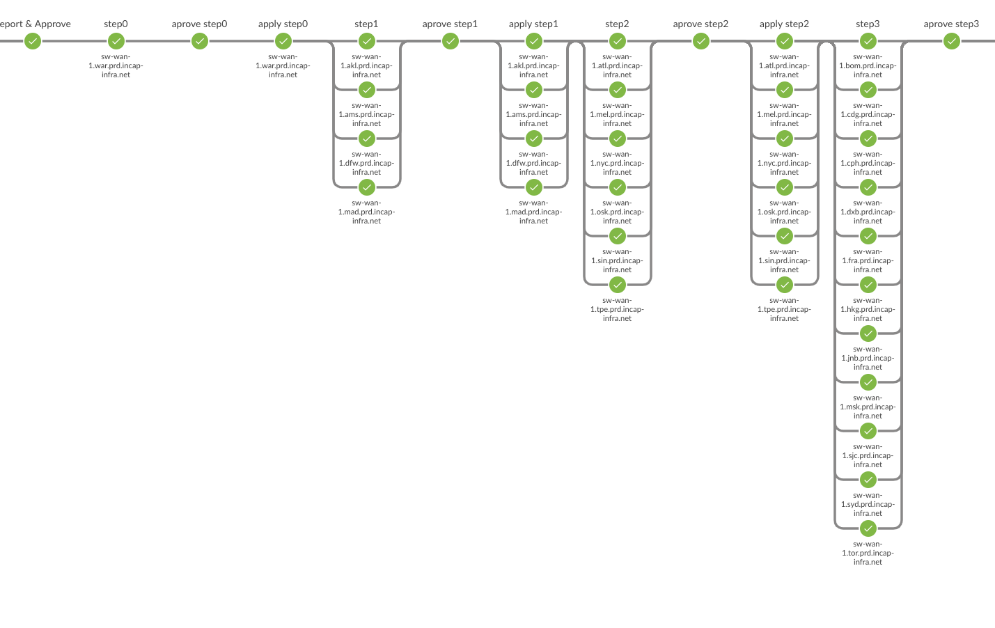
The deployment system we built is based on Jenkins. The deploy job merges configuration from the dev branch into the production branch, and triggers the deployment process, which is performed in multiple stages. In the first stage, we check which of the devices will be affected by the new configuration. According to the result we define steps for applying the configuration. In each step we deploy only to a subset of devices in order to reduce risk – the first step, for example, includes a small number of PoPs starting with the smallest and concluding with the largest. Between each step we monitor the network for stability to ensure we don’t cause any impact.
Here you can see part of the screenshot of our deployment process:
The monitoring process
Even though the deployment procedure is well-defined and could be run easily, the reality is, we need to monitor our devices regularly. Many cases, such as emergency issues or live debug sessions, require manual configuration on the devices, but we need to ensure that this will be cleaned up at the end. The other aspect of the job is to validate that what’s committed to the production is indeed deployed into the devices.
So, at any given time we want to validate two things:
- Our Git repo is in sync with production (single source of truth is indeed deployed to the devices).
- No manual configuration resides on the device.
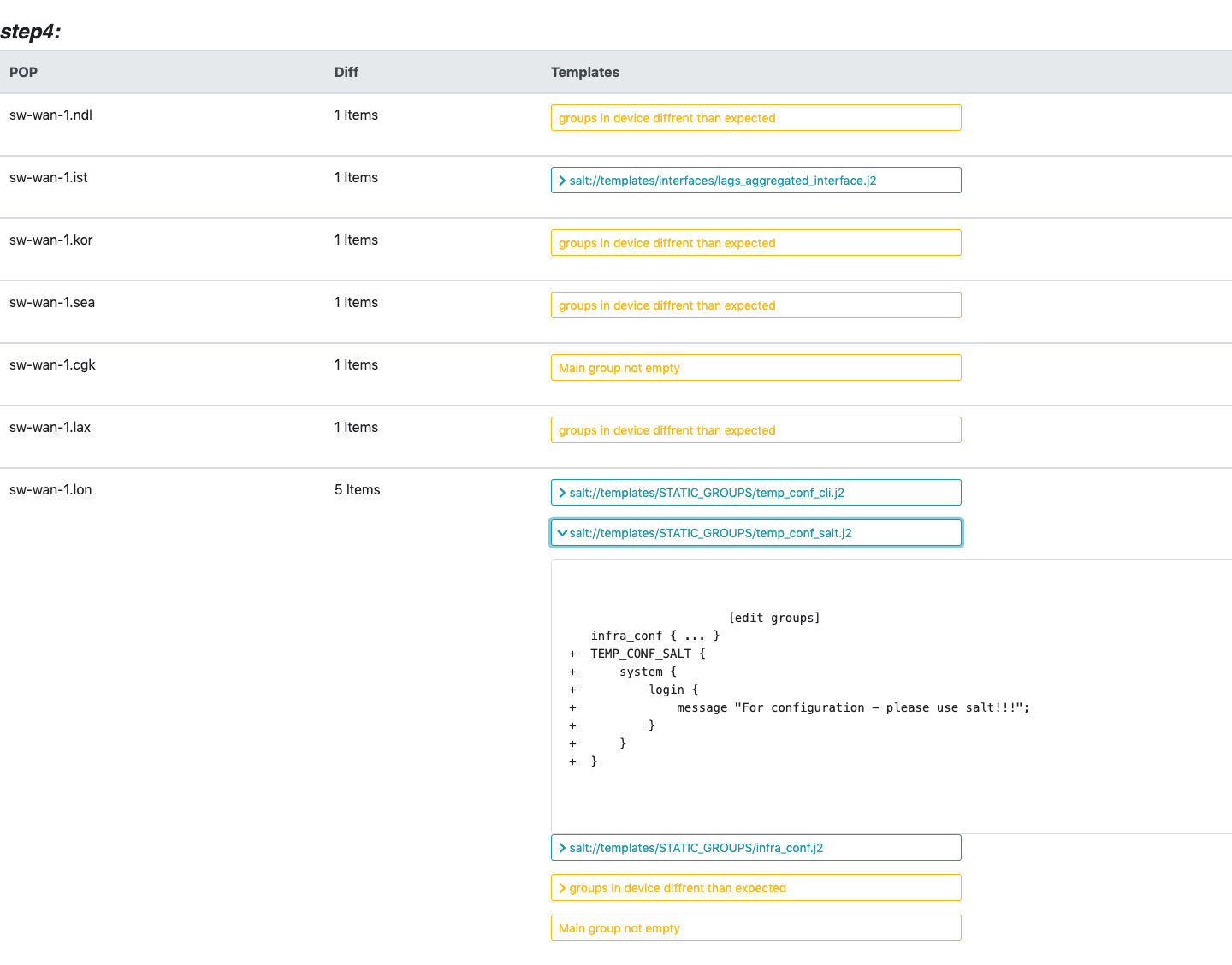
For this task we built another Jenkins job that runs periodically and performs the validation. The validation itself is performed using a Salt state that compares all templates that should be deployed on the device. The state validates that we have no diff inside the configuration namespaces, as well as validating that there’s no other unexpected configuration on the device outside of the namespaces. The results are analyzed by the Jenkins job and rendered into a nice html report that helps us understand the nature of the diff. In case a configuration mismatch is detected, the system will send an alert to the network engineering team with the reported attached.
Here you can see a diff report done during our rollout process, which explains the large number of diffs in the report. Each section in the report defines a diff – and you can expand it to see the actual mismatch.
Conclusion
Salt is a very cool system, and really helps us to find order among chaos. It has dramatically reduced the need for manual logins to the device, improved stability of our production environment and enabled us to build more automation on top of it.
On a team level, the change has enabled us to focus on automation rather than manually maintaining production. The team has evolved from an operations team to a development team, investing most of our time in developing networking automation.
To limit the length of this blog, I’ve only described parts of what we’ve already done. My feeling is that we’ll learn more and more use cases as we continue to scale. One of my team members soon intends to post a blog about how we handle congested provider pipes in our cloud. I’m sure you can’t wait!
The post Adding Some Salt to Our Network – Part 2 appeared first on Blog.
*** This is a Security Bloggers Network syndicated blog from Blog authored by Eyal Leshem. Read the original post at: https://www.imperva.com/blog/adding-some-salt-to-our-network-part-2/
