

Great Expectations
Thus far, the situations we have modeled have been either
over-simplifications or fabrications in order to illustrate a concept.
This article will try to improve on that a bit by considering more
variables and closer to reality, too. We will do so by presenting the
subject matter needed to understand and review the article An
Adversarial Risk Analysis Framework for Cybersecurity by Insua et al
(2019), still in preprint form.
They say a picture is worth a thousand words, and that applies to risk
analysis as well. Besides the obvious examples of mathematical plots,
diagrams can be great aids in understanding and modeling a situation
whose outcome is unknown. Remember tree
diagrams? They are a good
tool to help understand a situation in which there are several choices
and one depends on the other. In reality, they are a simplified version
of Bayesian
Networks.
In both, the number joining two random events gives the probability of
the end node happening, if we already know the origin node happened.
But not all random situations in life are entirely random. Some are
decisions which should be taken strategically, taking into account all
the information at hand. In the 1970s, decision theorists extended such
diagrams to involve such rational decisions and their consequences in
terms of rewards or penalties (utilities), which rational agents are
supposed to maximize.
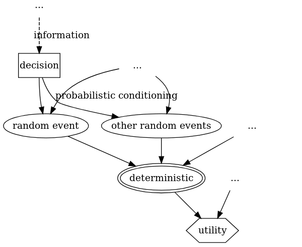
Figure 1. Diagram
In this influence diagram, solid arrows indicate that the node at the
tip depends probabilistically on the node at the tail. As illustrated by
each node label:
rectangles are for decisions to be made by rational agents,
sometimes based on information which can depend on the occurrence of
a random event or another choice;ellipses are for random events, typically costs associated with a
particular riskdouble ellipses for deterministic situations (usually a mathematical
function of the random events, tipically used for costs that depend
on them),and hexagons represent the utility, reward or penalty associated
with such an outcome.
Influence diagrams can be a lot more complicated, but for now that will
suffice. Notice how decisions are at the first level. Depending on those
decisions, some random events (typically costs associated with a
particular risk) will happen or not, that’s another level. From the
outcomes of those random events, a deterministic function (usually the
total of the costs) is computed and from that, a utility is computed.
Also, influence diagrams can involve more than one decision-making
agent, which can be distinguished using colors.
With that in mind, the following model for cybersecurity attacks can be
easily understood:
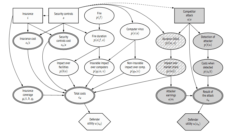
Figure 2. Influence diagram for a cybersecurity situation
It looks a bit busy, but bear with us. Keep in mind the layer
arrangement described above, ignore all the mathematical notation and
focus only on the shapes and labels. There are two players involved: the
defender and attacker. The attacker has to decide whether or not to
launch an attack (row 1), depending on the information they gain about
the defender’s decision to implement security controls. The defender
might choose to acquire insurance for their cyber assets. Each party has
a utility node (last row), each of which depends on the deterministic
nodes (row 4) which sum up the results of random impacts (row 3), which
depend on random events (row 2). That is, in a nutshell, an influence
diagram for cyber warfare.
Mathematical interlude: expectation
Another important concept to understand this model is that of expected
value. As it name implies, it is the value that can be reasonably
expected for a random variable, taking into account the probability of
each value, i.e., its distribution. However the mathematical formula to
compute it doesn’t look too user friendly, so it deserves some
explanation.
The expected value is not unlike an average taken from a sample. Say you
want the average age of people in a room:
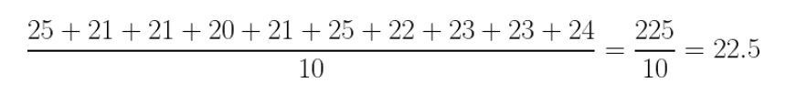
Figure 3. Average 1
So, if you had to guess a person’s age, it would make sense to go for 22
o 23. But adding like that would be too much work for large samples. Why
not group them instead, count how many are each age, and weight each
value with that count?
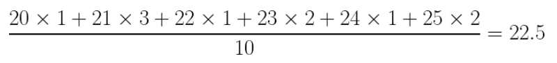
Figure 4. Average 2
This can be interpreted in terms of probabilities. If we break up that
fraction, we can rewrite that sum as
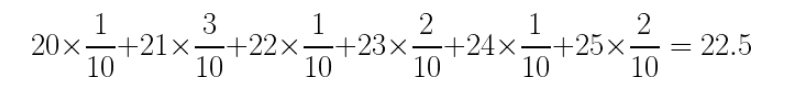
Figure 5. Average 3
Which is nothing more than the sum of each value times its probability.
This is just the definition of expected value for a discrete probability
distribution:
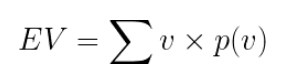
Figure 6. Expected Value Discrete
where v is each value, p(v) is its probability, and the sums runs
over all possible values. For continuous distributions, the sum over all
values is upgraded to a integral over all values:
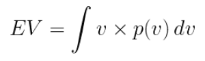
Figure 7. Expected Value Continuous Distribution
Back to the model
We would like to compute and maximize the expected value for the
utility, but that value depends probabilistically on others. Recalling
our discussion about conditional probability, you
know that the probability of two events happening together can be
computed with the probability of one of them, and the probability of one
given the other. If we have a chain of events, each depending on the
last, that rule would imply a succession of multiplied conditional
probabilities:

Figure 8. Expected Utility
I know this looks like crazy math, but focus on the product of
conditional probabilities. All that is just the probability of having
the utility u corresponding to the parameters cn,
ct, cc, etc. According to the above discussion
of expected value, we just multiply the value by its probability and
integrate.
Now that we have an estimate of expected utility, we need only simulate
and throw some optimization algorithms to obtain the maximum values and
which parameters (the decisions, the configuration, etc) that give us
that maximum value. In the above model, where what needs to be decided
is whether to acquire insurance and security controls, for the defender,
and the attacker needs to decide whether to launch an attack, the
results of running such simulations and optimizations are that the
defender should get the best-in-class, 1 terabyte per second,
cloud-based DDos protection, implement a firewall and anti-fire
system, and subscribe to comprehensive cyberattack insurance. Not too
surprising.
Having understood both concepts above, plus the optimization algorithms
we will not go into, because they would take us too far away from the
main topic, all of which are standard mathematical topics, the article
can be understood. In the original, however, we are walked through every
addition to the model step by step, beginning from a simple model where
utility depends from a single random node, adding one piece at a time.
This might be good from a pedagogical point of view, but we feel it
would be more valuable to explain the conventions for influence diagrams
as we did above. Also they first build a few reusable abstract model.
There is nothing special about “fire” above. It is a risk just like an
earthquake or robbery. Only the probability distribution and the impact
values would change. Likewise “virus” and “DDos” could mean any kind of
untargeted and targeted cybersecurity risk, respectively.
After having presented the general model, the authors go to great
lengths to explain every detail of the use case model (the above
diagram), including definitions of what each term (such as “DDos” or
“confidentiality”) mean. At the very end end they rush through the
results, discussion and conclusions. So, in terms of reviewing the
paper, we feel that it is overly long in the obvious, and lacking in the
difficult to grasp or most valuable. Personally, I feel this is not
research proper, but merely a novel application of well-established
topics to a particular game theoretic situation which might apply to
cybersecurity as it could to any other attack-defense scenario.
References
- D. Rios, A. Couce, J. Rubio, W. Pieters, K. Labunets, D. Garcia
(2019). An Adversarial Risk Analysis Framework for Cybersecurity.
arXiv preprint
*** This is a Security Bloggers Network syndicated blog from Fluid Attacks RSS Feed authored by Rafael Ballestas. Read the original post at: https://fluidattacks.com/blog/great-expectations/
