Home » Security Bloggers Network » Serverless ETLs? Easy Data Lake Transformations using AWS Athena

Serverless ETLs? Easy Data Lake Transformations using AWS Athena

by Ori Nakar on December 25, 2019

In a data lake raw data is added with little or no processing, allowing you to query it straight away. This gives you a great way to learn about your data – whether it represents a quick win or a fast fall. However, there are two disadvantages: performance and costs.

If, for example you added CSV files to your object store and created an external table, there’s no difference in the size of scanned data for these two queries:

SELECT COUNT(1)
FROM csv_based_table

SELECT *
FROM csv_based_table
ORDER BY 1

In AWS Athena the scanned data is what you pay for, and you wouldn’t want to pay too much, or wait for the query to finish, when you can simply count the number of records.

In this post we’ll explore the importance of transformations, and how they can be done.

In October 2018, AWS announced support for Creating Tables using the results of a Select query (CTAS). PrestoDB, the core of Athena, Google’s Big Query and Apache Spark have all supported the same functionality for a long time and there’s a good reason why.

Sponsorships Available

The heavy work is done by Athena, and the solution can be completely serverless by using AWS Lambda or AWS Glue to perform a set of queries.

We’ll explain when it’s possible to use CTAS for transformations, and how using it improved our daily work and processes.

Data lake queries

Data collected and stored in the data lake is constantly ready to be explored. The table’s metadata (sometimes called catalog) contains the following information:

Data location and folder structure
Files format
Record structure

After a table is added, data can be queried. Here’s an example of an external table creation:

CREATE EXTERNAL TABLE my_table (
 id   bigint,
 name string)
ROW FORMAT DELIMITED
 FIELDS TERMINATED BY ','
LOCATION 's3://my-bucket/my-folder'
TBLPROPERTIES ('skip.header.line.count'='1')

In this example “my_table” will be used to query CSV files under the given S3 location.

You can also run AWS Glue Crawler to create a table according to the data you have in a given location.

Exploration is a great way to know your data. And when a use case is found, data should be transformed to improve user experience and performance.

Transformations

Transformation goals are to:

Improve user experience
Improve performance
Reduce costs

Depending on the use case, it’s possible to achieve these goals by:

Filtering unwanted data, extracting relevant fields
Aggregating data to reduce its size and make analysis easier
Sorting and indexing the data

Before CTAS we had to iterate the query results which were written to a CSV file by Athena. We then had to convert the results to parquet files. Fortunately, there’s now no need for this unnecessary write and read to S3. Using CTAS has made transformations easier, and dramatically reduced the time it takes to transform the data.

Use-cases and examples

Here are some use cases and examples of how CTAS can be used to transform your data.

Use-case 1 – Filter and aggregate data

This is the simplest and most common use of CTAS – creating your own copy of the relevant data you need for your work:

CREATE TABLE new_table
WITH (external_location='s3://my-bucket/tables/my-table-location',) 
AS
 SELECT usecase_column1, usecase_column2
 FROM table1 INNER JOIN table2 ON ...
 WHERE filter_condition
 GROUP BY usecase_aggregation

In this example the table created allows working with the filtered data without specifying the filter again and again. The query engine doesn’t use the larger table, which can improve performance and reduce costs. While this is a simple example we have much complex example using the processing power of Athena:

SQL WITH clause for programmatic queries, map reduce and reuse of calculation data
Presto built in aggregation queries, including approximate functions which allows large calculations with small memory footprint
Presto window functions

Use-case 2 – Convert format

Improve your query performance and reduce your Athena and S3 costs by converting your data to Columnar Storage Formats. Here’s an example for how it can be done using CTAS:

# create an external table based on JSON files
CREATE EXTERNAL TABLE my_csv_table (
 id   bigint,
 name struct<first_name:string,last_name:string>)
ROW FORMAT SERDE 
  'org.openx.data.jsonserde.JsonSerDe' 
LOCATION 's3://my-bucket/my-folder'

# convert to parquet and flatten JSON
CREATE TABLE my_parquet_table
WITH (
 format = 'Parquet',
 external_location='s3://my-bucket/tables/my-table-location'
) AS SELECT id,first_name, last_name 
    FROM my_csv_table

If, for example, you query only specific columns, you can see how this simple conversion dramatically reduces the data scanned. This example also shows how we flatten a JSON structure, it is possible to do more complex operation JSON maps and arrays – see array and maps functions in the presto documentation.

Use-case 3 – Index data

Indexing the data is probably the most efficient way to improve performance and reduce costs. For example, if you’re using partitions, only data in the wanted partitions will be scanned. Here’s an example of how a daily partition can be implemented:

# create a partitioned table
CREATE EXTERNAL TABLE my_table (
 col1 string,
 col2 string)
PARTITIONED BY (
 day string)
STORED PARQUET
LOCATION 's3://my-bucket/tables/my-table-location'

# load partitions from file systems
# if there is a folder under the table location called day=2019-01-01
#  it will be added as a partition
MSCK REPAIR TABLE my_table

# query the partition, only data under the folder will be scanner
SELECT COUNT(1)
FROM my_table
WHERE day = '2019-01-01'

With CTAS you can create a partitioned table, in which each value in the partitioned column will have its own folder:

CREATE TABLE my_partitioned_table
WITH (
 format = 'Parquet',
 external_location='s3://my-bucket/tables/my-table-location',
 partitioned_by = ARRAY['my_partition_column']       
) AS SELECT col1, col2, ... my_partition_column
     FROM my_table

Partitioning is an effective way of reducing the scanned data. Although it’s limited, you can partition by more than one column and have up to 100 partitions. And should your column have high cardinality and evenly distributed values you can use bucketing instead of partitioning. Bucketing will split the data into the number of files (the bucket) you specify. The query engine knows how to access the right file according to the searched value. You can find more examples in the AWS Athena documentation, including a comparison of partitioning and bucketing.

Data flow

In this example, data is constantly added to the data lake, and we’d like to transform that incoming data. The flow has three main steps: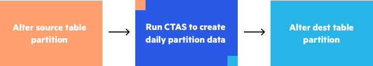

Here’s an example of how we use CTAS as ETL – creating a daily table partition using CTAS, then transforming the existing table with the new partition:

# alter source table(s) with partition
ALTER TABLE my_source_table
ADD IF NOT EXISTS PARTITION (day='2019-01-01')
LOCATION 's3://my-bucket/source-data/day=2019-01-20/'

# use ctas to create daily partition. 
# In this example table also has a ‘type’ partition
CREATE TABLE temp_ctas_table
WITH (
format = 'Parquet',
external_location='s3://my-bucket/tables/my-location/day=2019-01-20/',
partitioned_by = ARRAY['type']
) AS SELECT col1, col2, type
    FROM my_source_table
    WHERE day='2019-01-01'

# drop created table
DROP TABLE temp_ctas_table

# alter dest table with new partitions
ALTER TABLE my_table
ADD IF NOT EXISTS
PARTITION (day='2019-01-01', type=1)
LOCATION 's3://my-bucket/tables/my-location/day=2019-01-20/type=1'
PARTITION (day='2019-01-01', type=2)
LOCATION 's3://my-bucket/tables/my-location/day=2019-01-20/type=2'

This flow demonstrates how ETLs processes – whether simple or complex – can be done by using several SQL commands.

Takeaway

SQL is a great way to query data and, unlike many Big Data solutions, is supported by Athena . Together with CTAS, it can be used for research and, as seen in this post, for production ETLs. Finally, since it can be used from the AWS console, it’s really easy to try it on your own data. Why not give it a go?

The post Serverless ETLs? Easy Data Lake Transformations using AWS Athena appeared first on Blog.