
Fool the Machine
Artificial Neural Networks (ANNs) are certainly a wondrous
achievement. They solve classification and other learning tasks with
great accuracy. However, they are not flawless and might misclassify
certain inputs. No problem, some error is expected. But what if you
could give it two inputs that are virtually identical, but you get
different outputs? Worse, what if one is correctly classified but the
other has been manipulated so that it is classified as anything you
want? Could these adversarial examples be the bane of neural networks?
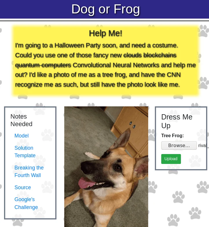
That is what happened with one PicoCTF challenge
we came across recently. There is an application whose sole purpose is
to accept a user-uploaded image, classify it, and let you know the
results. Our task was to take the image of a dog, correctly classified
as a Malinois, and manipulate it so that it is classified as a tree
frog. However, for your image to be a proper adversarial example, it
must be perceptually indistinguishable from the original, in other
words, it must still look like the same previously-classified dog to a
human.
The applications are potentially endless. You could:


- fool image recognition systems like physical security cameras, as
does this Stealth
T-shirt.

- make an autonomous car crash.
- confuse virtual assistants.
- bypass spam filters, etc.
So, how does one go about creating such an adversarial example? Recall
that in our brief survey of machine learning techniques, we discussed
training neural
networks.
It is an iterative process in which you continuously adjust the weight
parameters of your black box (the ANN) until the outputs agree with
the expected ones, or at least, minimize the cost function, which is a
measure of how wrong the prediction is. I will borrow an image that
better explains it from an article by Adam Geitgey [2].
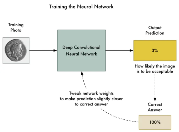
Figure 2. Training a neural network by [2].
This technique is known as backpropagation. Now, in order to obtain a
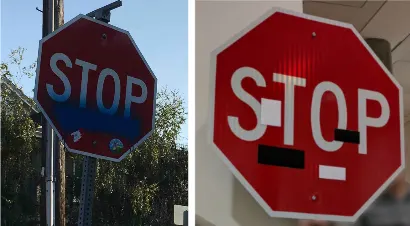
picture that is still like the original, but will classify as something
entirely different, what one could do is add some noise; but not too
much noise, so the picture doesn’t change, and not just anywhere, but
exactly in the right places, so that the classifier reads a different
pattern. Some clever folks from Google found out that the best way to do
this is by using the gradient of the cost function.
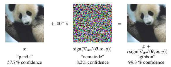
Figure 3. Adding noise to fool the classifier. From [1]
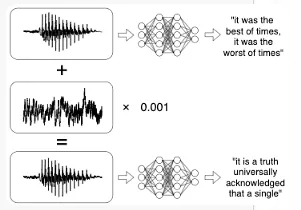
This is called the fast gradient sign method. This gradient can be
computed using backpropagation but in reverse. Since the model is
already trained, and we can’t modify it, let’s modify the picture little
by little and see if it gets us any closer to the target. I will again
borrow from @ageitgey since the
analogy is much clearer this way.
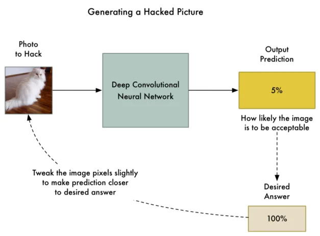
Figure 4. Tweaking the image, by [2].
The pseudo-code that would generate an adversarial example via this
method would be as follows. Assume that the model is saved in a Kerash5 file, as in the challenge. Keras is a
popular high-level neural networks API for Python. We can load the
model, get the input and output layers (first and last), get the cost
and gradient functions and define a convenience function that returns
both for a particular input, like this:
Getting cost function and gradients from a neural network.
from keras.models import load_modelfrom keras import backend as Kmodel = load_model('model.h5')input_layer = model.layers[0].inputoutput_layer = model.layers[-1].outputcost_function = output_layer[0, object_type_to_fake]gradient_function = K.gradients(cost_function, input_layer)[0]get_cost_and_gradients = K.function([input_layer, K.learning_phase()], [cost_function, gradient_function])Where object_type_to_fake is the class number of what we want to fake.
Now, according to the formula in figure 3 above, we should add a small
fraction of the sign of the gradient, until we achieve the result. The
result should be that the confidence in the prediction becomes at least
95%.
while confidence < 0.95: cost, gradient = get_cost_and_gradients([adversarial_image, 0]) adversarial_image += 0.007 * np.sign(gradient)However, this procedure takes way too long without a GPU. A few hours
according to Geitgey [2]. For the CTFer and the more
practical-minded reader, there is a library that does this and other
attacks on machine learning systems to determine their vulnerability to
adversarial examples:
CleverHans. Using this
library, we change the expensive while cycle above to two API calls:
make an instance of the attack method and then ask it to generate the
adversarial example.
from cleverhans.attacks import MomentumIterativeMethodmethod = MomentumIterativeMethod(model, sess=K.get_session())test = method.generate_np(adversarial_image, eps=0.3, eps_iter=0.06, nb_iter=10, y_target=target)In this case, we used a different attack, namely theMomentumIterativeMethod because, in this situation, it gives better
results than the FastGradientMethod, obviously also a part ofCleverHans. And so we obtain our adversarial example.
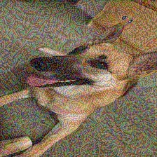
Figure 5. Adversarial image for the challenge
You can almost see the tree frog lurking in the back, if you imagine
the two knobs on the cabinet are its eyes. Just kidding. Upload it to
the challenge site and, instead of getting the predictions, we get the
flag.
Not just that, the model which is based onMobileNet,
is 99.99974% certain that this is a tree frog. However, the difference
between it and the original image, according to the widely used
perceptual hash algorithm, is less than two bits. Still, the adversarial
example has artifacts, at least to a human observer.
What is worse is that these issues persist across different models as
long as the training data is similar. That means that we could probably
pass the same image to a different animal image classifier and still get
the same results.
Ultimately, we should think twice before deploying ML-powered security
measures. This is, of course, a mock example, but in more critical
situations, having models that are not resistant to adversarial examples
could result in catastrophic effects. Apparently[1],
the reason behind this is the linearity within the functions hidden in
these networks. So switching to a more non-linear model, such as RBF
networks,
could solve the problem. Another workaround could be to train the ANNs
including adversarial examples.
To borrow a phrase from carpenters, “Measure twice, cut once.” We should
also remember that whatever the solution, it should be clear that one
should test twice, and deploy once.
References
I. Goodfellow, J. Shlens, C. Szegedy. EXPLAINING AND HARNESSING
ADVERSARIAL EXAMPLES. arXiv.A. Geigtey. Machine Learning is Fun Part 8: How to Intentionally
Trick Neural Networks.
Medium
*** This is a Security Bloggers Network syndicated blog from Fluid Attacks RSS Feed authored by Rafael Ballestas. Read the original post at: https://fluidattacks.com/blog/fool-machine/