
Vulnerability Modeling with Binary Ninja
This is Part 3 in a series of posts about the Binary Ninja Intermediate Language (BNIL) family. You can read Part 1 here and Part 2 here.
In my previous post, I demonstrated how to leverage the Low Level IL (LLIL) to write an architecture-agnostic plugin that could devirtualize C++ virtual functions. A lot of new and exciting features have been added to Binary Ninja since then; in particular, Medium Level IL (MLIL) and Single Static Assignment (SSA) form[1]. In this post, I’m going to discuss both of these and demonstrate one fun use of them: automated vulnerability discovery.
Plenty of static analyzers can perform vulnerability discovery on source code, but what if you only have the binary? How can we model a vulnerability and then check a binary to see if it is vulnerable? The short answer: use Binary Ninja’s MLIL and SSA form. Together, they make it easy to build and solve a system of equations with a theorem prover that takes binaries and turns them, alchemy-like, into vulnerabilities!
Let’s walk through the process with everyone’s favorite hyped vulnerability of yesteryear, Heartbleed.
Hacking like it’s 2014: Let’s find Heartbleed!
For those who might not remember or be familiar with the Heartbleed vulnerability, let’s run through a quick refresher. Heartbleed was a remote information-disclosure vulnerability in OpenSSL 1.0.1 – 1.0.1f that allowed an attacker to send a crafted TLS heartbeat message to any service using TLS. The message would trick the service into responding with up to 64KB of uninitialized data, which could contain sensitive information such as private cryptographic keys or personal data. This was possible because OpenSSL used a field in the attacker’s message as a size parameter for malloc and memcpy calls without first validating that the given size was less than or equal to the size of the data to read. Here’s a snippet of the vulnerable code in OpenSSL 1.0.1f, from tls1_process_heartbeat:


 /* Read type and payload length first */
    hbtype = *p++;
    n2s(p, payload);
    pl = p;

    /* Skip some stuff... */

    if (hbtype == TLS1_HB_REQUEST)
        {
        unsigned char *buffer, *bp;
        int r;

        /* Allocate memory for the response, size is 1 bytes
         * message type, plus 2 bytes payload length, plus
         * payload, plus padding
         */
        buffer = OPENSSL_malloc(1 + 2 + payload + padding);
        bp = buffer;

        /* Enter response type, length and copy payload */
        *bp++ = TLS1_HB_RESPONSE;
        s2n(payload, bp);
        memcpy(bp, pl, payload);
        bp += payload;
        /* Random padding */
        RAND_pseudo_bytes(bp, padding);

        r = ssl3_write_bytes(s, TLS1_RT_HEARTBEAT, buffer, 3 + payload + padding);
Looking at the code, we can see that the size parameter (payload) comes directly from the user-controlled TLS heartbeat message, is converted from network-byte order to host-byte order (n2s), and then passed to OPENSSL_malloc and memcpy with no validation. In this scenario, when a value for payload is greater than the data at pl, memcpy will overflow from the buffer starting at pl and begin reading the data that follows immediately after it, revealing data that it shouldn’t. The fix in 1.0.1g was pretty simple:
 hbtype = *p++;
    n2s(p, payload);
    if (1 + 2 + payload + 16 > s->s3->rrec.length)
        return 0; /* silently discard per RFC 6520 sec. 4 */
    pl = p;
This new check ensures that the memcpy won’t overflow into different data.
Back in 2014, Andrew blogged about writing a clang analyzer plugin that could find vulnerabilities like Heartbleed. A clang analyzer plugin runs on source code, though; how could we find the same vulnerability in a binary if we didn’t have the source for it? One way: build a model of a vulnerability by representing MLIL variables as a set of constraints and solving them with a theorem prover!
Model binary code as equations with z3
A theorem prover lets us construct a system of equations and:
- Verify whether those equations contradict each other.
- Find values that make the equations work.
For example, if we have the following equations:
x + y = 8
2x + 3 = 7
A theorem prover could tell us that a) a solution does exist for these equations, meaning that they don’t contradict each other, and b) a solution to these equations is x = 2 and y = 6.
For the purposes of this exercise, I’ll be using the Z3 Theorem Prover from Microsoft Research. Using the z3 Python library, the above example would look like the following:
>>> from z3 import *
>>> x = Int('x')
>>> y = Int('y')
>>> s = Solver()
>>> s.add(x + y == 8)
>>> s.add(2*x + 3 == 7)
>>> s.check()
sat
>>> s.model()
[x = 2, y = 6]
Z3 tells us that the equations can be satisfied and provides values to solve them. We can apply this technique to modeling a vulnerability. It turns out that assembly instructions can be modeled as algebraic statements. Take the following snippet of assembly:
  lea eax, [ebx+8]
  cmp eax, 0x20
  jle allocate
  int3
allocate:
  push eax
  call malloc
  ret
When we lift this assembly to Binary Ninja’s LLIL, we get the following graph:
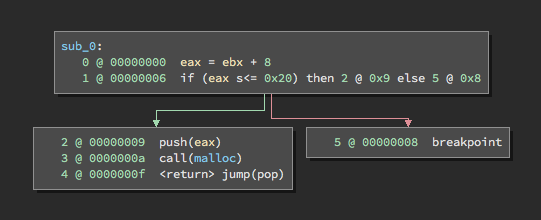
Figure 1. LLIL makes it easy to identify the signed comparison conditional.
In this code, eax takes the value of ebx and then adds 8 to it. If this value is above 0x20, an interrupt is raised. However, if the value is less than or equal to 0x20, the value is passed to malloc. We can use LLIL’s output to model this as a set of equations that should be unsatisfiable if an integer overflow is not possible (e.g. there should never be a value of ebx such that ebx is larger than 0x20 but eax is less than or equal to 0x20), which would look something like this:
eax = ebx + 8
ebx > 0x20
eax <= 0x20
What happens if we plug these equations into Z3? Not exactly what we’d hope for.
>>> eax = Int('eax')
>>> ebx = Int('ebx')
>>> s = Solver()
>>> s.add(eax == ebx + 8)
>>> s.add(ebx > 0x20)
>>> s.add(eax >> s.check()
unsat
There should be an integer overflow, but our equations were unsat. This is because the Int type (or “sort” in z3 parlance) represents a number in the set of all integers, which has a range of -∞ to +∞, and thus an overflow is not possible. Instead, we must use the BitVec sort, to represent each variable as a vector of 32 bits:
>>> eax = BitVec('eax', 32)
>>> ebx = BitVec('ebx', 32)
>>> s = Solver()
>>> s.add(eax == ebx + 8)
>>> s.add(ebx > 0x20)
>>> s.add(eax >> s.check()
sat
There’s the result we expected! With this result, Z3 tells us that it is possible for eax to overflow and call malloc with a value that is unexpected. With a few more lines, we can even see a possible value to satisfy these equations:
>>> s.model()
[ebx = 2147483640, eax = 2147483648]
>>> hex(2147483640)
'0x7ffffff8'
This works really well for registers, which can be trivially represented as discrete 32-bit variables. To represent memory accesses, we also need Z3’s Array sort, which can model regions of memory. However, stack variables reside in memory and are more difficult to model with a constraint solver. Instead, what if we could treat stack variables the same as registers in our model? We can easily do that with Binary Ninja’s Medium Level IL.
Medium Level IL
Just as LLIL abstracts native disassembly, Medium Level IL (MLIL) adds another layer of abstraction on top of LLIL. Whereas LLIL abstracted away flags and NOP instructions, MLIL abstracts away the stack, presenting both stack accesses and register accesses as variables. Additionally, during the process of mapping LLIL to MLIL, memory stores that aren’t referenced later are identified and eliminated. These processes can be observed in the example below. Notice how there are no stack accesses (i.e. push or pop instructions) and var_8 does not appear in the MLIL at all.

Figure 2a. An example function in x86.

Figure 2b. LLIL of the example function.

Figure 2c. MLIL of the example function.
Another feature you might notice in the MLIL is that variables are typed. Binary Ninja initially infers these types heuristically, but the user can override these with manual assignment later. Types are propagated through the function and also help inform the analysis when determining function signatures.
MLIL structure
Structurally, MLIL and LLIL are very similar; both are expression trees and share many of the same expression types for operations (for more on the IL’s tree structure, see my first blog post). However, there are several stark differences. Obviously, MLIL does not have analogous operations for LLIL_PUSH and LLIL_POP, since the stack has been abstracted. The LLIL_REG, LLIL_SET_REG, and other register-based operations are instead MLIL_VAR, MLIL_SET_VAR, and similar. On top of this, thanks to typing, MLIL also has a notion of structures; MLIL_VAR_FIELD and MLIL_STORE_STRUCT expressions describe these operations.
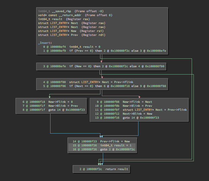
Figure 3. Types in MLIL can generate some very clean code.
Some operations are common to both LLIL and MLIL, though their operands differ. The LLIL_CALL operation has a single operand: dest, the target of the call. In contrast, the MLIL_CALL operation also specifies the output operand that identifies what variables receive a return value and the params operand, which holds a list of MLIL expressions that describe the function call’s parameters. A user-specific calling convention, or one determined by automated analysis based on usage of variables interprocedurally, determines these parameters and return values. This allows Binary Ninja to identify things like when the ebx register is used as a global data pointer in an x86 PIC binary, or when a custom calling convention is used.
Putting all of this together, MLIL comes pretty close to decompiled code. This also makes MLIL ideal for translating to Z3, due to its abstraction of both registers and stack variables, using Binary Ninja’s API.
MLIL and the API
Working with MLIL in the Binary Ninja API is similar to working with LLIL, though there are some notable differences. Like LLIL, a function’s MLIL can be accessed directly via the medium_level_il property of the Function class, but there is no corresponding MLIL method to get_low_level_il_at. In order to directly access a specific instruction’s MLIL, a user must first query for the LLIL. The LowLevelILInstruction class now has a medium_level_il property that retrieves its MediumLevelILInstruction form. As a single line of Python, this would look like current_function.get_low_level_il_at(address).medium_level_il. It is important to remember that this can sometimes be None, as an LLIL instruction can be optimized away completely in MLIL.
The MediumLevelILInstruction class introduces new convenience properties that aren’t available in the LowLevelILInstruction class. The vars_read and vars_written properties make it simple to query an instruction for a list of variables the instruction uses without parsing the operands. If we revisit an old instruction from my first blog post, lea eax, [edx+ecx*4], the equivalent MLIL instruction would look similar to the LLIL. In fact, it appears to be identical at first glance.
>>> current_function.medium_level_il[0]
<il: eax = ecx + (edx << 2)>
But, if we look closer, we can see the difference:
>>> current_function.medium_level_il[0].dest
<var int32_t* eax>
Unlike LLIL, where dest would have been an ILRegister object representing the register eax, the dest operand here is a typed Variable object, representing a variable named eax as an int32_t pointer.
There are several other new properties and methods introduced for MLIL as well. If we wanted to extract the variables read by this expression, this would be as simple as:
>>> current_function.medium_level_il[0].vars_read
[<var int32_t* ecx>, <var int32_t edx>]
The branch_dependence property returns the conditional branches of basic blocks that dominate the instruction’s basic block when only the true or false branch dominates, but not both. This is useful for determining which decisions an instruction explicitly depends on.
Two properties use the dataflow analysis to calculate the value of an MLIL expression: value can efficiently calculate constant values, and possible_values uses the more computationally-expensive path-sensitive dataflow analysis to calculate ranges and disjoint sets of values that an instruction can result in.

Figure 5. Path-sensitive dataflow analysis identifies all concrete data values that can reach a certain instruction.
With these features at our disposal, we can model registers, stack variables, and memory, but there is one more hangup that we need to solve: variables are often re-assigned values that are dependent on the previous value of the assignment. For example, if we are iterating over instructions and come across something like the following:
mov eax, ebx
lea eax, [ecx+eax*4]
When creating our equations, how do we model this kind of reassignment? We can’t just model it as:
eax = ebx
eax = ecx + (eax * 4)
This can cause all sorts of unsatisfiability, because constraints are purely expressing mathematical truths about variables in a system of equations and have no temporal element at all. Since constraint solving has no concept of time, we need to find some way to bridge this gap, transforming the program to effectively remove the idea of time. Moreover, we need to be able to efficiently determine from where the previous value eax originates. The final piece of the puzzle is another feature available via the Binary Ninja API: SSA Form.
Single Static Assignment (SSA) Form
In concert with Medium Level IL’s release, Binary Ninja also introduced Static Single Assignment (SSA) form for all representations in the BNIL family. SSA form is a representation of a program in which every variable is defined once and only once. If the variable is assigned a new value, a new “version” of that variable is defined instead. A simple example of this would be the following:
|
|
The other concept introduced with SSA form is the phi-function (or Φ). When a variable has a value that is dependent on the path the control flow took through the program, such as an if-statement or loop, a Φ-function represents all of the possible values that that variable could take. A new version of that variable is defined as the result of this function. Below is a more complicated (and specific) example, using a Φ-function:
|
|
SSA makes it easy to explicitly track all definitions and uses of a variable throughout the lifetime of the program, which is exactly what we need to model variable assignments in Z3.
SSA form in Binary Ninja
The SSA form of the IL can be viewed within Binary Ninja, but it’s not available by default. In order to view it, you must first check the “Enable plugin development debugging mode” box in the preferences. The SSA form, seen below, isn’t really meant to be consumed visually, as it’s more difficult to read than a normal IL graph. Instead, it is primarily intended to be used with the API.

Figure 6. An MLIL function (left) and its corresponding SSA form (right).
The SSA form of any of the intermediate languages is accessible in the API through the ssa_form property. This property is present in both function (e.g. LowLevelILFunction and MediumLevelILFunction) and instruction (e.g. LowLevelILInstruction and MediumLevelILInstruction) objects. In this form, operations such as MLIL_SET_VAR and MLIL_VAR are replaced with new operations, MLIL_SET_VAR_SSA and MLIL_VAR_SSA. These operations use SSAVariable operands instead of Variable operands. An SSAVariable object is a wrapper of its corresponding Variable, but with the added information of which version of the Variable it represents in SSA form. Going back to our previous re-assignment example, the MLIL SSA form would output the following:
eax#1 = ebx#0
eax#2 = ecx#0 + (eax#1 << 2)
This solves the problem of reusing variable identifiers, but there is still the issue of locating usage and definitions of variables. For this, we can use MediumLevelILFunction.get_ssa_var_uses and MediumLevelILFunction.get_ssa_var_definition, respectively (these methods are also members of the LowLevelILFunction class).
Now our bag of tools is complete, let’s dive into actually modeling a real world vulnerability in Binary Ninja!
Example script: Finding Heartbleed
Our approach will be very similar to Andrew’s, as well as the one Coverity used in their article on the subject. Byte-swapping operations are a pretty good indicator that the data is coming from the network and is user-controlled, so we will use Z3 to model memcpy operations and determine if the size parameter is a byte-swapped value.

Figure 7. A backward static slice of the size parameter of the vulnerable memcpy in tls1_process_heartbeat of OpenSSL 1.0.1f, in MLIL
Step 1: Finding our “sinks”
It would be time-consuming and expensive to perform typical source-to-sink taint tracking, as demonstrated in the aforementioned articles. Let’s do the reverse; identify all code references to the memcpy function and examine them.
    memcpy_refs = [
        (ref.function, ref.address)
        for ref in bv.get_code_refs(bv.symbols['_memcpy'].address)
    ]

    dangerous_calls = []

    for function, addr in memcpy_refs:
        call_instr = function.get_low_level_il_at(addr).medium_level_il
        if check_memcpy(call_instr.ssa_form):
            dangerous_calls.append((addr, call_instr.address))
Step 2: Eliminate sinks that we know aren’t vulnerable
In check_memcpy, we can quickly eliminate any size parameters that Binary Ninja’s dataflow can calculate on its own[2], using the MediumLevelILInstruction.possible_values property. We’ll model whatever is left.
def check_memcpy(memcpy_call):
    size_param = memcpy_call.params[2]

    if size_param.operation != MediumLevelILOperation.MLIL_VAR_SSA:
        return False

    possible_sizes = size_param.possible_values

    # Dataflow won't combine multiple possible values from
    # shifted bytes, so any value we care about will be
    # undetermined at this point. This might change in the future?
    if possible_sizes.type != RegisterValueType.UndeterminedValue:
        return False

    model = ByteSwapModeler(size_param, bv.address_size)

    return model.is_byte_swap()
Step 3: Track the variables the size depends on
Using the size parameter as a starting point, we use what is called a static backwards slice to trace backwards through the code and track all of the variables that the size parameter is dependent on.
        var_def = self.function.get_ssa_var_definition(self.var.src)

        # Visit statements that our variable directly depends on
        self.to_visit.append(var_def)

        while self.to_visit:
            idx = self.to_visit.pop()
            if idx is not None:
                self.visit(self.function[idx])
The visit method takes a MediumLevelILInstruction object and dispatches a different method depending on the value of the instruction’s operation field. Recalling that BNIL is a tree-based language, visitor methods will recursively call visit on an instruction’s operands until it reaches the terminating nodes of the tree. At that point it will generate a variable or constant for the Z3 model that will propagate back through the recursive callers, very similar to the vtable-navigator plugin of Part 2.
The visitor for MLIL_ADD is fairly simple, recursively generating its operands before returning the sum of the two:
    def visit_MLIL_ADD(self, expr):
        left = self.visit(expr.left)
        right = self.visit(expr.right)

        if None not in (left, right):
            return left + right
Step 4: Identify variables that might be part of a byte swap
MLIL_VAR_SSA, the operation that describes an SSAVariable, is a terminating node of an MLIL instruction tree. When we encounter a new SSA variable, we identify the instruction responsible for the definition of this variable, and add it to the set of instructions to visit as we slice backwards. Then, we generate a Z3 variable to represent this SSAVariable in our model. Finally, we query Binary Ninja’s range value analysis to see if this variable is constrained to being a single byte (i.e. within the range 0 – 0xff, starting at an offset that is a multiple of 8). If it is, we go ahead and constrain this variable to that value range in our model.
    def visit_MLIL_VAR_SSA(self, expr):
        if expr.src not in self.visited:
            var_def = expr.function.get_ssa_var_definition(expr.src)
            if var_def is not None:
                self.to_visit.append(var_def)

        src = create_BitVec(expr.src, expr.size)

        value_range = identify_byte(expr, self.function)
        if value_range is not None:
            self.solver.add(
                Or(
                    src == 0,
                    And(src = value_range.step)
                )
            )

            self.byte_vars.add(expr.src)

        return src
The parent operation of an MLIL instruction that we visit will generally be MLIL_SET_VAR_SSA or MLIL_SET_VAR_PHI. In visit_MLIL_SET_VAR_SSA, we can recursively generate a model for the src operand as usual, but the src operand of an MLIL_SET_VAR_PHI operation is a list of SSAVariable objects, representing each of the parameters of the Φ-function. We add each of these variables’ definition sites to our set of instructions to visit, then write an expression for our model that states dest == src0 || dest == src1 || … || dest == srcn:
        phi_values = []

        for var in expr.src:
            if var not in self.visited:
                var_def = self.function.get_ssa_var_definition(var)
                self.to_visit.append(var_def)

            src = create_BitVec(var, var.var.type.width)

            # ...

            phi_values.append(src)

        if phi_values:
            phi_expr = reduce(
                lambda i, j: Or(i, j), [dest == s for s in phi_values]
            )

            self.solver.add(phi_expr)
In both visit_MLIL_SET_VAR_SSA and visit_MLIL_SET_VAR_PHI, we keep track of variables that are constrained to a single byte, and which byte they are constrained to:
        # If this value can never be larger than a byte,
        # then it must be one of the bytes in our swap.
        # Add it to a list to check later.
        if src is not None and not isinstance(src, (int, long)):
            value_range = identify_byte(expr.src, self.function)
            if value_range is not None:
                self.solver.add(
                    Or(
                        src == 0,
                        And(src = value_range.step)
                    )
                )

                self.byte_vars.add(*expr.src.vars_read)

                if self.byte_values.get(
                    (value_range.step, value_range.end)
                ) is None:
                    self.byte_values[
                        (value_range.step, value_range.end)
                    ] = simplify(Extract(
                                int(math.floor(math.log(value_range.end, 2))),
                                int(math.floor(math.log(value_range.step, 2))),
                                src
                            )
                    )
And finally, once we’ve visited a variable’s definition instruction, we mark it as visited so that it won’t be added to to_visit again.
Step 5: Identify constraints on the size parameter
Once we’ve sliced the size parameter and located potential bytes used in our byte swap, we need to make sure that there aren’t any constraints that would restrict the value of the size on the path of execution leading to the memcpy. The branch_dependence property of the memcpy’s MediumLevelILInstruction object identifies mandatory control flow decisions required to arrive at the instruction, as well as which branch (true/false) must be taken. We examine the variables checked by each branch decision, as well as the dependencies of those variables. If there is a decision made based on any of the bytes we determined to be in our swap, we’ll assume this size parameter is constrained and bail on its analysis.
        for i, branch in self.var.branch_dependence.iteritems():
            for vr in self.function[i].vars_read:
                if vr in self.byte_vars:
                    raise ModelIsConstrained()
                vr_def = self.function.get_ssa_var_definition(vr)
                if vr_def is None:
                    continue
                for vr_vr in self.function[vr_def].vars_read:
                    if vr_vr in self.byte_vars:
                        raise ModelIsConstrained
Step 6: Solve the model
If the size isn’t constrained and we’ve found that the size parameter relies on variables that are just bytes, we need to add one final equation to our Z3 Solver. To identify a byte swap, we need to make sure that even though our size parameter is unconstrained, the size is still explicitly constructed only from the bytes that we previously identified. Additionally, we also want to make sure that the reverse of the size parameter is equal to the identified bytes reversed. If we just added an equation to the model for those properties, it wouldn’t work, though. Theorem checkers only care if any value satisfies the equations, not all values, so this presents a problem.
We can overcome this problem by negating the final equation. By telling the theorem solver that we want to ensure that no value satisfies the negation and looking for an unsat result, we can find the size parameters that satisfy the original (not negated) equation for all values. So if our model is unsatisfiable after we add this equation, then we have found a size parameter that is a byte swap. This might be a bug!
           self.solver.add(
                Not(
                    And(
                        var == ZeroExt(
                            var.size() - len(ordering)*8,
                            Concat(*ordering)
                        ),
                        reverse_var == ZeroExt(
                            reverse_var.size() - reversed_ordering.size(),
                            reversed_ordering
                        )
                    )
                )
            )

            if self.solver.check() == unsat:
                return True
Step 7: Find bugs
I tested my script on two versions of OpenSSL: first the vulnerable 1.0.1f, and then 1.0.1g, which fixed the vulnerability. I compiled both versions on macOS with the command ./Configure darwin-i386-cc to get a 32-bit x86 version. When the script is run on 1.0.1f, we get the following:

Figure 8. find_heartbleed.py successfully identifies both vulnerable Heartbleed functions in 1.0.1f.
If we then run the script on the patched version, 1.0.1g:

Figure 9. The vulnerable functions are no longer identified in the patched 1.0.1g!
As we can see, the patched version that removes the Heartbleed vulnerability is no longer flagged by our model!
Conclusion
I’ve now covered how the Heartbleed flaw led to a major information leak bug in OpenSSL, and how Binary Ninja’s Medium Level IL and SSA form translates seamlessly to a constraint solver like Z3. Putting it all together, I demonstrated how a vulnerability such as Heartbleed can be accurately modeled in a binary. You can find the script in its entirety here.
Of course, a static model such as this can only go so far. For more complicated program modeling, such as interprocedural analysis and loops, explore constraint solving with a symbolic execution engine such as our open source tool Manticore.
Now that you know how to leverage the IL for vulnerability analysis, hop into the Binary Ninja Slack and share with the community your own tools, and if you’re interested in learning even more about the BNIL, SSA form, and other good stuff.
Finally, don’t miss the Binary Ninja workshop at Infiltrate 2018. I’ll be hanging around with the Vector 35 team and helping answer questions!
[1] After Part 2, Jordan told me that Rusty remarked, “Josh could really use SSA form.” Since SSA form is now available, I’ve added a refactored and more concise version of the article’s script here!
[2] This is currently only true because Binary Ninja’s dataflow does not calculate the union of disparate value ranges, such as using bitwise-or to concatenate two bytes as happens in a byte swap. I believe this is a design tradeoff for speed. If Vector 35 ever implements a full algebraic solver, this could change, and a new heuristic would be necessary.
*** This is a Security Bloggers Network syndicated blog from Trail of Bits Blog authored by Josh Watson. Read the original post at: https://blog.trailofbits.com/2018/04/04/vulnerability-modeling-with-binary-ninja/